Negative Mass and Negative Refractive Index in Atom Nuclei - Nuclear Wave Equation - Gravitational and Inertial Control -(Part 1)- Physics Answers

Raul Fattore

April 7, 2023

The present study is divided into six parts

Abstract

Some efforts have been made to prove negative mass behavior through some experiments performed in mechanics [1], and other disciplines [9], as well as some theories in electrostatics [2,3,4,5,6,7,8], but I haven’t found research about similar effects at the atomic level, where the most elementary mass given by the atomic nucleus is to be found.

Is the second Newton’s law still valid with negative mass?
What could happen if we make the atom behave in a negative mass regime?
Is the negative refractive index related to negative mass?
Are we able to control the magnitude of mass?
Are we able to control the sign of mass?

The answers to these questions are given through this series of papers, with results that are coincident with experimental data, except for the negative mass regime. Experiments must be done to confirm or invalidate the theory developed in these articles. Needless to say, if experiments validate this theory, then a significant change in mankind is going to happen. In that case, I strongly ask scientists to cooperate by making use of the derived technologies for good and refrain from doing it for evil.

Introduction

The theory presented in these papers is based on three fundamental aspects that have proved to be extremely effective to describe physical phenomena and predicting results that agree with experimental data [10, 11, 12]:

• Spinning Ring Model of Elementary Particles (toroidal ring of continuous charge)
• New Atomic Model
• The Universal Electrodynamic Force

Figure 1
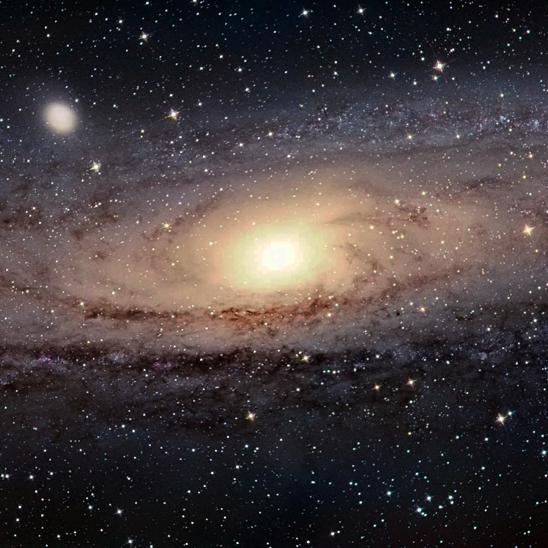
Bostick’s toroidal charge fiber ring

As a result of some experiments in 1919, Compton found out that the electron cannot be a sphere of charge but a “ring of electricity” [13]. Bostick, who was one of his students, published a torus model for particles in 1956 (Fig. 1). Since then, the toroidal ring model of particles has been further improved by David L. Bergman and J. Paul Wesley in 1990 [10, 14]. The spinning ring model of elementary particles is superior to any previous quantum models. The three main characteristics of the ring model are: the real physical size of the particle, the magnetic dipole behavior of the particle, and the lack of continuous radiation of a spinning ring with static electric and magnetic fields.

The concept of “point particle” is a mere mathematical help used in Quantum Mechanics and Relativity Theory that does not account for real-size particles in the real world.

Figure 2
Example of atomic particle arrangement

An outcome of the spinning ring of elementary particles was a new atomic model proposed by Joseph Lucas and Charles W. Lucas, Jr. in 2002 [11]. This new atomic model is not only based on theory but also checked with simple practical experiments that explain how the elementary particles might be packed in the atom according to the balance of electromagnetic forces (Fig. 2).

This new atomic model is based on the finite size of particles, their internal structure, and the elastic deformation they may undergo. Quantum Mechanics and Relativity Theory both ignore these facts. The model is more fundamental than any previous atomic models, including the planetary one, that violates Ampere’s and Faraday’s laws for orbiting electrons (they are required to radiate, lose energy, and fall towards the nucleus, which will collapse the atom).

Electrons in the new atomic model do not orbit the nucleus. They are positioned at a stable equilibrium distance from it due to the balance of electromagnetic forces.

Figure 3
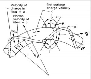
Charge density of proton and neutron

The new atomic model predicts how electrons are organized in shells. Moreover, it also predicts a shell’s organization of nucleons. We know that the nucleus contains two types of particles: protons and neutrons.

Neutrons are stable in the nucleus. However, outside the nucleus, the neutron decays into a proton and an electron with a half-life of fewer than 15 minutes. The mass of the neutron is the sum of the masses of the electron and proton. The neutron has a charge density that varies between positive and negative with respect to its radius (Fig. 3). These facts suggest that the neutron might not be a valid elementary particle, but a bound combination of an electron with a proton [15].

Accordingly, the new atomic model precisely describes how electrons and protons are very tightly packed in shells in the nucleus due to the balance of electromagnetic forces.

As previously mentioned, the last fundamental aspect these papers are based on is the Universal Electrodynamic Force. Here we have two options: the universal force from Wilhelm Weber’s theory of electrodynamics (1846 and 1848), and the universal force derived more recently (2006 and 2007) by Charles W. Lucas, Jr. [12].

Weber’s universal force showed for the first time the appearance of the constant “c” (speed of light), which was a function of the material parameters (permittivity and permeability) as we know it today. From Weber’s universal force, one can derive the Coulomb law, Ampere’s law, Newton’s second law, Newton’s gravitational law, etc. Unfortunately, Helmholtz objected to a negative sign in the second term of the equation, meaning “that a charge behaves somewhat as if its mass were negative so that in certain circumstances its velocity might increase indefinitely under the action of a force opposed to the motion”. Because of this objection, Weber’s force was discredited and abandoned.

Weber’s universal force is based on the relative motion of two charges and was a tremendous advance at that time. Unfortunately, there are two factors that prevent a practical use of that equation: it is an action-at-a-distance force (instantaneous action at any distance, like Newton’s laws), and the lack of a radiation term.

Lucas’ universal force, on the other hand, is derived from the fundamental empirical equations of electrodynamics, which are solved simultaneously by the method of substitution using the Galilean transformation.

Figure 4
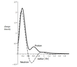
Relative motion only depends on relative coordinates

This force, which is also based on the relative motion of two charges, is entirely relational, and whatever we measure from this motion will have the same value in all frames of reference. That’s why the traditional Galilean transformation is used. It is a real relativistic theory because it only depends on relative coordinates instead of relative reference frames. Einstein’s relativity theory and Lorentz’s transformation become useless and invalid in such a real, natural environment. Moreover, Einstein’s relativity theory is totally unnecessary, because it is a theory that is far from physical reality.

This universal force should be considered a fundamental equation in physics. It tells us how mother nature works, from the macro world to the atomic level. It is not an action-at-a-distance force. It is based on finite size, elastic particles, and self-fields. It uses Galilean transformation based on causality. It always conserves energy and momentum, satisfies Mach’s principle, and has chiral symmetry. Furthermore, it is really relativistic because it only depends on relative coordinates instead of relative reference frames.

From this universal force, one can derive many equations, for example, forces that are superior to Newton’s second law and Newton’s gravitational law, the centrifugal force, the equation of mass, all electrostatic and electrodynamics laws, the radiation, radiation reaction forces, and more.

The Universal Force Law

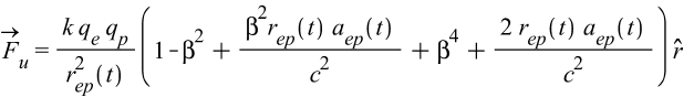
Luca’s universal electrodynamic force in vectorial form is:

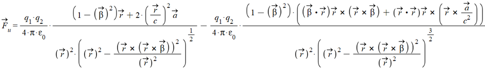
Where $\vec{\beta}=\frac{\vec{v}}{c}$ , and $\vec{r},\ \vec{v},\ \vec{a}$ , are the relative position, velocity, and acceleration between the two charges.

Figure 5
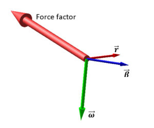
Force factor from the triple vectorial product

The triple vectorial products in the second term, involving the velocity and the acceleration, give rise to a helical motion of the particles (corkscrew motion).

These terms are absent in Newton’s laws, and explain the centrifugal force, the drift in the orbit of some planets, and the gyroscopic drifts.

The result is a circular motion with tangential velocity $\vec{\beta}=\frac{\vec{v}}{c}$ and acceleration $\frac{\vec{a}}{c^2}$ , and a force pointing outwards which is perpendicular to the displacement $\vec{r}$ (Fig. 5).

Figure 6
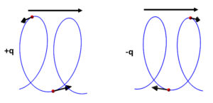
Helical motion of charges given by the force factor

This is nothing else than the centrifugal force component or the equivalent radial acceleration, which is equal and opposite to the centripetal acceleration. When $\vec{r}$ changes with time, this motion will describe a helix or spiral in the direction of the motion. If the particles are charges, the rotation direction will depend on the sign of the charges (Fig. 6).

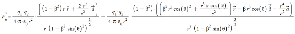
In general, velocity and acceleration may not have the same direction. Let’s define their angles with respect to the vector $\vec{r}$ .

$\theta$ : angle between $\vec{r}$ and $\vec{v}$

$\alpha$ : angle between $\vec{r}$ and $\vec{a}$

We can write the universal force in the geometrical form:

A Connected Universe under Continuous Radiation

Every particle in the universe is under the influence of all the others. There is an endless dynamic interchange of energy. Nothing is isolated, and nothing is at rest. We can only mathematically simulate these last two states to study the self-behavior of a particle, but we need to add an external agent to better understand how a particle behaves in boundary-limited environments.

Since zero-degree Kelvin it is not known to be reached in the universe, it is safe to assume that the elementary particles in the atom always vibrate, and the atom radiate continuously, sending an electromagnetic field to other atoms. Then, every atom in the universe will “process” the received energy, which could be partially absorbed, totally absorbed, or not absorbed at all.

All these fields fill what we know as the “space” among all particles. “Space” is a concept, and we cannot “bend” a concept as Einstein proposed, but we can “bend” the electromagnetic fields.

The continuous vibrational state of elementary particles is also a base for the present study.

Forces in Atom Nuclei

For this study, I have chosen the Aluminum atom, which is a material easy to find anywhere and can be used for several purposes, in case experiments validate the results obtained here.

The mass of the atom is 99.9% given by its nucleus. As mentioned before, the neutron is a bound between an electron and a proton, and they are organized in tight-packed shells in the nucleus. The main contribution to the atomic mass is given by protons, since they have a mass about 1840 times greater than electrons. The proton radius is about $0.84\ {10}^{-15}\ [m]$ , while the electron radius is approximately $2.81\ {10}^{-15}\ [m]$ . However, these particles heavily shrink when they are bound, and expand when they are unbound. Therefore, we can only speak of average size.

The aluminum atom has atomic number Z=13 and atomic mass A=27. We know that the atomic mass gives the number of protons and neutrons in the nucleus, that is, there are 13 protons plus 14 neutrons. Since the neutron is a bound of an electron and a proton, we have in the nucleus 14 electrons plus 14 protons plus 13 protons, i.e., a total of 14 electrons and 27 protons.

Figure 7
One possible arrangement of shells for Aluminum nucleus

One possible configuration of the nuclear shells for Aluminum is shown in Fig. 7.

However, the particles will naturally group in shells in such a way as to balance magnetic and electric forces by finding a minimum, stable distance among them.

The balance of electric and magnetic forces in the nucleus causes the nucleons to rearrange to form a minimum number of shells, and the innermost shells to break up to form larger, more stable shells.

Figure 8
Adopted shell arrangement for Aluminum atomic nucleus

Therefore, I assume the shells’ organization for the nucleus shown in Fig. 8.

This sandwich configuration keeps the particles very tightly bound together. Note that at three shells in from the outermost shell, there are always two proton shells in a row for the larger nuclides. This weak binding allows the outermost sandwich of shells to have liquid-like properties and forms the proper justification for a Liquid Drop Model of the nucleus.

As we already know, the torus ring model of the particles has an associated electric field as well as a magnetic field. However, due to the very tight packing configuration of the particles, we may safely assume that the distance among shells is extremely tiny and that the predominant force in the nucleus is of electrostatic origin, while the weaker magnetic forces will add some contribution to the equilibrium distance between each shell.

Coulomb Force Among Nuclear Shells

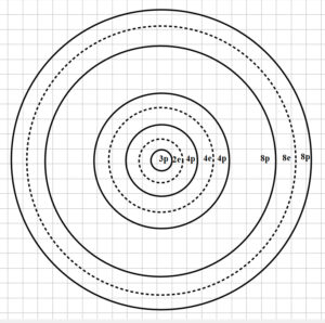
The new atomic model shows us a discrete distribution of particles around big circles which do not constitute real shells (see Fig. 2). But for the sake of simplicity, assume that the big circles can be replaced by shells, with the charge homogeneously distributed on their surface.

The net Coulomb Force is the sum of the interaction of a shell with all the others. The number of terms $n$ of the force is given by the combination of all cross products between 2 shells: $C=\frac{n!}{2!\ (n-2)!}$ .

That means we are going to have 15 terms for the force in our 6 shells structure.

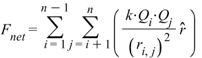
${\vec{F}}{net}={\vec{F}}_1+{\vec{F}}_2+{\vec{F}}_3+…{\vec{F}}{15}$

The net force for 6 shells with total charge per shell $Q_i$ and $Q_j$ , and a distance $r_{i,j}$ between a shell pair, is given by the following formula:

(3)

(4)

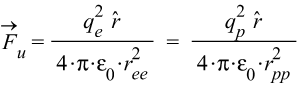
Where $q_p$ is the proton charge, and $q_e$ is the electron charge.

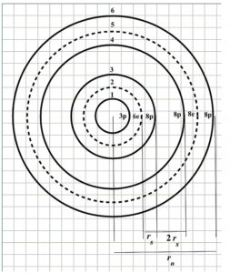
Averaging the distance between two shells

Calculating the electrostatic equilibrium distance of the nuclear arrangement for such a number of shells is a very heavy algebraic process. The need for powerful computational capacities, which I don’t have, is mandatory. Anyhow, for the arrangement given in Fig. 8, we can make a rough average estimation that might easily be within the real distance value with a reasonable error.

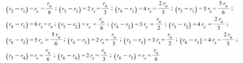
Before averaging all the distances, we must make a very simplistic assumption regarding the distances between shells to work with just one “estimated” distance $r_s$ (Fig. 8). This distance is taken from the origin to the 1st proton shell ( $r_{01}=r_s$ ) to be the same as each distance p-e and e-p in the “sandwich” shells. In other words, we assume that all shells are equidistant, that is $r_s=\frac{r_n}{6}$ , where $r_n$ is the nucleus radius. We assume that the distance between the two successive proton shells is $2\ r_s$ . Then, the combination of all 15 distances between shell pairs will be:

Adding up all these distances gives $r_{sum}=7.33\ r_n$ . Then, the mean linear distance between any two shells is $r_{12Avg}=\frac{r_{sum}}{15}=0.489\ r_n$ . To obtain the average distance in the volume of the nucleus, we must integrate this value over the whole nucleus volume. Our function to be integrated is $f_{(r)}=0.489\ r$ .

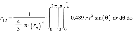
Which gives us the average distance between any two shells:

$r_{12}\cong0.37\ r_n$ (5)

Nuclear Shells Oscillations

As mentioned earlier, the focus of this analysis is on the atomic nucleus, which is where the atomic mass resides.

It was previously assumed that elementary particles always vibrate in the atom. Despite the extremely tight packing in the nucleus, and the huge Coulomb interaction forces, we may assume that proton and electron shells oscillate at some frequency, with a certain amplitude.

Figure 9
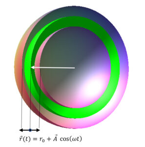
Scheme of an oscillating shell about the equilibrium position (green)

Assume that shell oscillation is radial so that shells will expand and shrink around a middle radius at a certain frequency (Fig. 9). The green shell shows the equilibrium position. For simplicity, suppose that the amplitude of the oscillation of all the electron shells is equal and that the amplitude of the oscillation of all the proton shells is also equal. We can express this mathematically for proton (p) and electron (e) shells as follows:

${\vec{r}}_p(t)={\vec{r}}_p+{\vec{A}}_p\ cos(\omega_pt+\emptyset_p)\ \ =\ \ r_p\hat{r}+A_p\ cos(\omega_pt+\emptyset_p)\ \hat{r}$ (6)

${\vec{r}}_e(t)={\vec{r}}_e+{\vec{A}}_e\ cos(\omega_et+\emptyset_e)\ \ \ =\ \ r_e\hat{r}+A_e\ cos(\omega_et+\emptyset_e)\ \hat{r}$ (7)

Where $r_p$ and $r_e$ are constants, and $A_p$ , $A_e$ is the maximum amplitude of oscillation of proton and electron shells respectively. To simplify these equations, we may arbitrarily set the initial phases to zero for $t=0$ , i.e., $\emptyset_p=\emptyset_e=0$ :

${\vec{r}}_p(t)={\vec{r}}_p+{\vec{A}}_p\ cos(\omega_pt)\ \ =\ \ r_p\hat{r}+A_p\ cos(\omega_pt)\ \hat{r}$ (8)

${\vec{r}}_e(t)={\vec{r}}_e+{\vec{A}}_e\ cos(\omega_et)\ \ \ =\ \ r_e\hat{r}+A_e\ cos(\omega_et)\ \hat{r}$ (9)

The velocity of oscillation of the proton and electron shells is given by the time derivative of (8) and (9).

$v_p=\frac{d{\vec{r}}_p(t)}{dt}\ =\ A_p{\ \omega}_p\ sin(\omega_pt)$

$v_e=\frac{d{\vec{r}}_e(t)}{dt}\ =\ A_e{\ \omega}_e\ sin(\omega_et)$

The maximum velocity is reached when the sinus function is equal to $\pm\ 1$ .

$v_p={\pm\ A}_p{\ \omega}_p$

$v_e={\pm\ A}_e{\ \omega}_e$

According to Eq. (4), we need the equations that account for the distance between equal and opposite charge shells.

Electron-Proton Shell Pair

${\vec{r}}_{ep}(t)=({\vec{r}}_e-{\vec{r}}_p)+({\vec{A}}_e\ cos(\omega_et)-\ {\vec{A}}_p\ cos(\omega_pt))\ \ =\ \ (r_e-r_p)\ \hat{r}+(A_e\ cos(\omega_et)-A_p\ cos(\omega_pt))\ \hat{r}$

The magnitude is:

$r_{ep}(t)=(r_e-r_p)+(A_e\ cos(\omega_et)-A_p\ cos(\omega_pt))$ (10)

The relative velocity between the shells is the time derivative of Eq. (10).

${\vec{v}}{ep}=\frac{d{\vec{r}}{ep}\left(t\right)}{dt}\ =\ \left{{\left(A\right}_p\ \omega}_p\ sin\left(\omega_pt\right)-A_e\ \omega_e\ sin\left(\omega_et\right)\right)\ \hat{r}$

The magnitude of the velocity after simplifying is:

$v_{ep}=A_e{\ \omega}_e\ sin(\omega_et)-A_p{\ \omega}_p\ sin(\omega_pt)$ (11)

The relative acceleration is:

${\vec{a}}{ep}=\frac{d{\vec{v}}{ep}(t)}{dt}\ =\ {(A}_p{{\ \omega}_p}^2\ cos(\omega_pt)-A_e{{\ \omega}_e}^2\ cos(\omega_et))\ \hat{r}$

The magnitude of the acceleration after simplifying is:

$a_{ep}=A_e{{\ \omega}_e}^2\ cos(\omega_et)-A_p{{\ \omega}_p}^2\ cos(\omega_pt)$ (12)

Proton-Proton Shell Pair

${\vec{r}}{pp}(t)=({\vec{r}}{p2}-{\vec{r}}{p1})+({\vec{A}}_p\ cos(\omega_pt)-\ {\vec{A}}_p\ cos(\omega_pt))\ \ =\ \ (r{p2}-r_{p1})\ \hat{r}$ (13)

The magnitude is:

$r_{pp}=(r_{p2}-r_{p1})$ (14)

The relative velocity and acceleration between proton shells are zero (time derivative of Eq. (13), which is a constant value).

${\vec{v}}_{pp}=0$ (15)

${\vec{a}}_{pp}=0$ (16)

Electron-Electron Shell Pair

${\vec{r}}{ee}(t)=({\vec{r}}{e2}-{\vec{r}}{e1})+({\vec{A}}_e\ cos(\omega_et)-\ {\vec{A}}_e\ cos(\omega_et))\ \ =\ \ (r{e2}-r_{e1})\ \hat{r}$ (17)

$r_{ee}=(r_{e2}-r_{e1})$ (18)

The relative velocity and acceleration between electron shells are zero (time derivative of Eq. (17), which is a constant value).

${\vec{v}}_{ee}=0$ (19)

${\vec{a}}_{ee}=0$ (20)

According to the interaction among shells described above, we need to be careful when applying the universal force to Eq. (4). We must use the proper expressions of the universal force as follows:

The relative velocity and acceleration between shells with equal charge signs are zero. For these terms in Eq. (4), we must apply the Universal Force for $v=0$ ( $a=0$ ).
The relative velocity and acceleration between shells with different charge signs are not zero. For these terms in Eq. (4), we must apply the Universal Force for $a\neq0$ .

The Universal Force for a ≠ 0

As explained above, this version of the force is to be applied for interactions of shells with different charge signs, that is, the force between e-p shell pairs in Eq. (4).

(21)

$\beta=\frac{v_{ep}(t)}{c}$

$k=\frac{1}{4\ \pi\ \varepsilon_0}$

The Universal Force for v=0 (a = 0)

This version of the force must be applied for interactions of shells with equal charge signs, i.e., the force between e-e and p-p shell pairs in Eq. (4).

(22)

In this case, the distance between the shells is a constant value, so we must use the averaged distance value:

$r_{ee}=r_{pp}\cong0.37\ r_n$ (see Eq. (5))

$r_n$ : nucleus radius

Applying the Universal Force to obtain the Nuclear Net Force

Now we can add up the 15 terms of the net Coulomb force given by Eq. (4) by applying the prior considerations to the corresponding terms. As the proton and electron charges are equal, we can write $q_e=q_p=q$ .

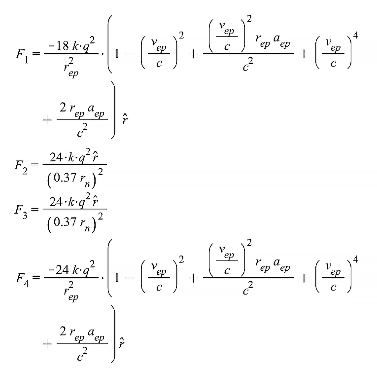
…….. and so on, until $F_{15}$ .

The final expression of the nuclear force is:

${\vec{F}}{net}=-\frac{378k\thinsp q^2}{r{ep}^2\left(t\right)}\left(1-\frac{v_{ep}^2\left(t\right)}{c^2}+\frac{v_{ep}^2\left(t\right)r_{ep}\left(t\right)a_{ep}\left(t\right)}{c^4}+\frac{v_{ep}^4\left(t\right)}{c^4}+\frac{2r_{ep}\left(t\right)a_{ep}\left(t\right)}{c^2}\right)\hat{r}+\frac{2279.035793k\thinsp q^2\hat{r}}{r_n^2}$ (23)

We see that the last term is independent of time. It’s an electrostatic term due to the interaction of shells having charges of the equal sign.

The Nuclear Net Force in terms of the Refractive Index

The net nuclear force can be written in terms of the index of refraction. Since the refractive index is given by the ratio of the speed of light with the velocity of the wave in the medium $n=\frac{c}{v_{ep}(t)}$ , we replace this value in the net force to get

${\vec{F}}{net}=-\frac{378k\thinsp q^2}{r{ep}^2\left(t\right)}\left(1-\frac{1}{n^2}+\frac{v_{ep}^2\left(t\right)r_{ep}\left(t\right)a_{ep}\left(t\right)}{n^2c^2}+\frac{1}{n^4}+\frac{2r_{ep}\left(t\right)a_{ep}\left(t\right)}{c^2}\right)\hat{r}+\frac{2279.035793k\thinsp q^2\hat{r}}{r_n^2}$ (23a)

Mass is not a Fundamental Quantity

From the second Newton’s law, we know that mass is always a positive constant value given by the ratio of the acting force and the resultant acceleration of a particle.

$m=\frac{\vec{F}}{\vec{a}}$

This positive constant appears in other equations, such as $E=mc^2$ , linear momentum, kinetic energy, etc.

In Newton’s gravitational law, both interacting masses are also positive quantities. It is always an attractive force.

$\vec{F}=-\ G\ \frac{m_1\ m_2}{{r_{12}}^2}$

However, according to the Universal Force Law, mass is not constant, but is a function of the elementary charges, and the amplitude and frequency of their oscillations. Its value can be modified at will, it can be made null, forced to adopt any magnitude, and its sign can be changed. Therefore, we cannot assume anymore that mass is a fundamental quantity. Thus, the ratio between force and acceleration acquires another significance, as well as the gravitational law.

In a negative mass regime, the direction of the acceleration opposes that of the force. The implications of this fact are unthinkable. The interaction between two particles (or bodies) can be forced to adopt any of the following three states: attraction, repulsion, or equilibrium.

The Intrinsic Nuclear Mass

As stated in previous paragraphs, since zero-degree Kelvin it is not known to be reached in the universe, it is safe to assume that the elementary particles in the atom are in a perpetual oscillatory motion. As the vibrations are permanent, and happen at any temperature, we may disregard the “cause” as an external agent and assume that the shell vibrations exist as a universal process of energy interchange since the creation of the atoms, and never stop.

Therefore, we may consider the nuclear shells as a “self-vibrating system” to analyze their intrinsic properties.

We may study the behavior of the nuclear mass by relating the internal nuclear net force ${\vec{F}}_{net}$ (Eq. 23) with the shells’ acceleration. As we have seen before, the acceleration is mainly given by the interaction between electron and proton shells ${\vec{a}}_{ep}$ .

${\vec{F}}{net}=m_n\ {\vec{a}}{ep}$ => $F_{net}\hat{r}=m_n\ a_{ep}\ \hat{r}$ => $m_n=\frac{F_{net}}{a_{ep}}$ (24)

$m_n=-\frac{378k\thinsp q^2}{r_{ep}^2\left(t\right)a_{ep}\left(t\right)}\left(1-\frac{v_{ep}^2\left(t\right)}{c^2}+\frac{v_{ep}^2\left(t\right)r_{ep}\left(t\right)a_{ep}\left(t\right)}{c^4}+\frac{v_{ep}^4\left(t\right)}{c^4}+\frac{2r_{ep}\left(t\right)a_{ep}\left(t\right)}{c^2}\right)+\frac{2279.035793k\thinsp q^2}{r_n^2a_{ep}\left(t\right)}$ (25)

Where:

$r_{ep}\left(t\right)=\left(0.37r_n+A_e\cos{\left(\omega_et\right)}-A_p\cos{\left(\omega_pt\right)}\right)$

$v_{ep}\left(t\right)=\left(-A_e\omega_e\sin{\left(\omega_et\right)}+A_p\sin{\left(\omega_pt\right)}\omega_p\right)$

$a_{ep}\left(t\right)=\left(-A_e\omega_e^2\cos{\left(\omega_et\right)}+A_p\omega_p^2\cos{\left(\omega_pt\right)}\right)$

Figure 10
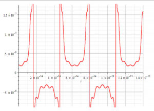
Graph showing negative mass during half periods

The radius of the nucleus of the aluminum atom is about $r_n=3.5\ fm\ =\ 3.5\ {10}^{-15}m$ . Amplitudes should be a small percentage of the nucleus radius, while the frequencies will depend on if they are caused by thermal effect, or by forced external oscillations from a certain agent. For now, we may assume that the time of oscillation of the shells has the same value and make some plots of the nuclear mass.

Figure 10 is a graph of the nuclear mass with respect to time, for the following parameters:

$r_n=3.5\ {10}^{-15}[m]$ ; $\omega_e={10}^{14}[\frac{1}{s}]$ ; $\omega_p={10}^{15}[\frac{1}{s}]$ ; $A_e=3.5\ {10}^{-17}[m]$ ; $A_p={10}^{-3}A_e[m]$

The frequency of oscillation in this case is:

$f=1.6\ {10}^{13}\ [Hz]$

Note that in this case, the Universal Force predicts negative mass during half a cycle.

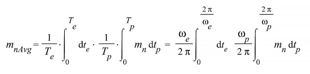
Time-Averaged Nuclear Mass

To obtain an expression of mass independent of time, we may assume different oscillation times for proton and electron shells and take a time average.

$r_{ep}\left(t\right)=\left(0.37r_n+A_e\cos{\left(\omega_et_e\right)}-A_p\cos{\left(\omega_pt_p\right)}\right)$

$v_{ep}\left(t\right)=\left(-A_e\omega_e\sin{\left(\omega_et_e\right)}+A_p\sin{\left(\omega_pt_p\right)}\omega_p\right)$

$a_{ep}\left(t\right)=\left(-A_e\omega_e^2\cos{\left(\omega_et_e\right)}+A_p\omega_p^2\cos{\left(\omega_pt_p\right)}\right)$

We need to replace these expressions in the mass formula to proceed with the averaging.

The time average is calculated over the period of each oscillation frequency. To make the integration easier, we may first take a Taylor series expansion on the variables $t_e$ and $t_p$ . Due to the nature of the mass equation and the singularities, it is recommended to expand it for 15 or more terms. Otherwise, the results might not be satisfactory. If you count with high computation capabilities, take as many terms as you can process.

(27)

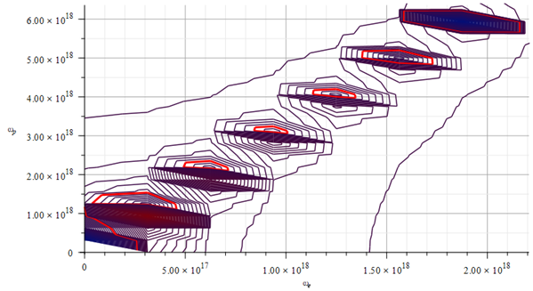
Figure 11 shows the contour plot of the mass (or levels’ plot) for electron and proton oscillation frequencies, according to the following parameters: $r_n=3.5\ {10}^{-15}[m]$ , $A_e=2\ {10}^{-16}[m]$ , $A_p={10}^{-3}A_e[m]$ . To ease the job to the computer, a Taylor expansion of 16 terms for $m_n$ was made on the variables $t_e$ and $t_p$ before integration.

Figure 11
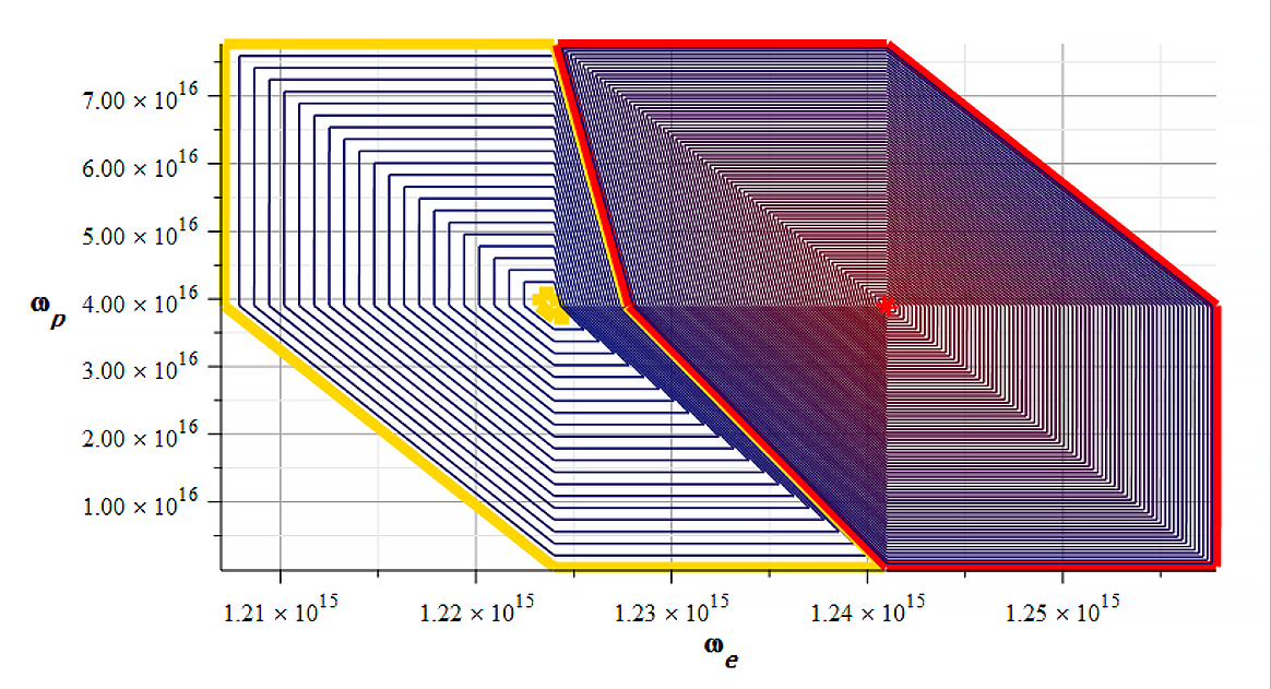
Mass level graph. Big red and yellow contours enclose negative and positive mass respectively

The red line encloses negative mass ranging from ~ $-1.8\ {10}^8[Kg]$ (red line) to $-1.7\ {10}^{10}[Kg]$ in the red dot (smallest contour).

The yellow line encloses positive mass ranging from ~ $3.8\ {10}^7[Kg]$ (yellow line) to $4.5\ {10}^9[Kg]$ in the yellow dot (smallest contour). Note the huge values of the mass for each sign.

Figure 12 shows the mass level plot with the same parameters as before, but for a different frequency range.

Figure 12
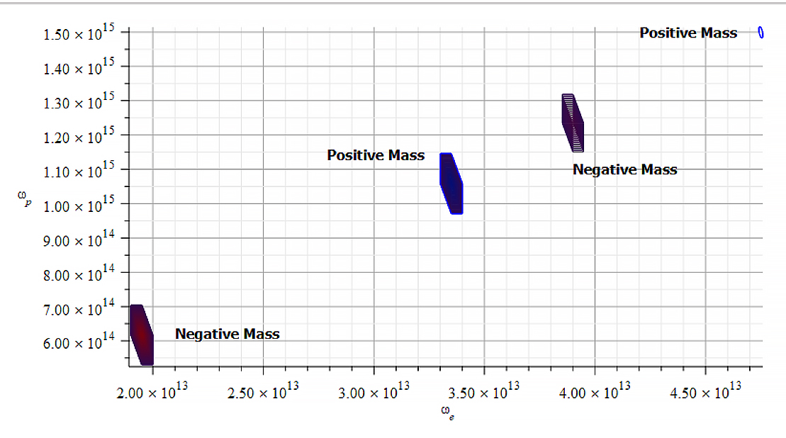
Mass level graph for a different frequency range as in Fig. 11, showing a periodic change on mass sign

In this case, the positive mass varies from ~ $8.5\ {10}^{17}[Kg]$ to $1.5\ {10}^{20}[Kg]$ , while the negative mass goes from $-\ 3.3\ {10}^{18}[Kg]$ to $-\ 2.6\ {10}^{20}[Kg]$ .

Note in this case that the values of mass are highly sensitive with frequencies $\omega_e$ and $\omega_p$ , being more critical for $\omega_e$ .

Note the linear periodic change of mass sign with proton and electron frequencies.

Fourier Analysis of the Nuclear Mass

We can make a frequency analysis of the mass (Eq. 25) with the parameters used for Fig. 10 to find the main frequency and its harmonics. The Fast Fourier Transform (FFT) was calculated with these parameters:

Total number of samples $N=2^{13}$ , sampling frequency $f_s=2^3\ f_p$ (proton frequency), which gives a frequency resolution $\Delta_{f}=\frac{f_s}{N}=1.55{10}^{11}\left[Hz\right]$ and a total acquisition time of $T=\frac{N}{f_s}=6.43\ {10}^{-12}[s]$ . The frequency at the i-sample number on the plot is determined by $f=\frac{N_{(i)}}{T}\ [Hz]$ .

Figure 13
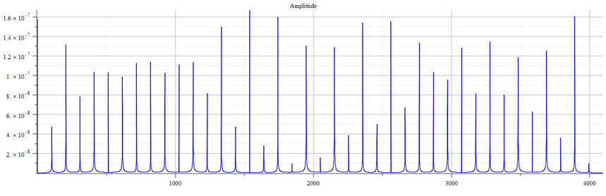
Fast Fourier Transform (FFT) amplitude graph vs. frequency of Eq. 25, with the parameters used in Fig. 10

Figure 14
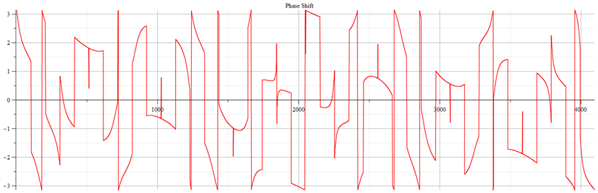
Fast Fourier Transform (FFT) phase shift graph corresponding to Fig. 13

The main frequency is $f_0=1.6\ {10}^{13}[Hz]$ . The following formula can be used to calculate the harmonics: $f=f_0+n\ f_0\ ;\ n=0,\ 1,\ 2,\ 3…$

Note in the phase plot the swings of phase between ±π, which are characteristic of resonance.

The “standard” mass of the Aluminum atom

According to the Commission on Isotopic Abundances and Atomic Weights (CIAAW), which is a worldwide authority on the atomic weights of elements, the Aluminum atom has an atomic mass of 26.9815384(3) Da, or the equivalent in kilogram to:

$m_{Al}=4.48\ {10}^{-26}\ [Kg]$ (28)

Since the nucleus contributes more than 99.9% to the atomic mass, we can safely take the same value for the nuclear mass of Aluminum.

However, according to the intrinsic nuclear mass previously defined, its value depends on the amplitude and frequency of the proton and electron shell oscillations. That is, the averaged intrinsic mass can be expressed as

$m=f(A_e,\ \omega_e,\ A_p,\ \omega_p)$ (29)

How can we have a “standard” value of mass then?

The answer is that there will always be a combination of those variables satisfying the “standard” mass value. Electrons and protons which are organized as nuclear shells (Fig. 7 and 8), are kept together by extremely strong electromagnetic forces, which automatically adapt the oscillatory variables to maintain the equilibrium among the shells, and the global equilibrium of the atom under natural circumstances. These electromagnetic forces inside the nucleus always seek the “natural” oscillatory equilibrium among shells to maintain a constant relationship of the mass variables given in Eq. (29). That’s the reason we measure the same constant value of mass under natural circumstances.

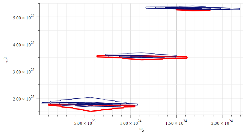
We don’t know the value of the amplitude of the oscillation of the shells. However, we may estimate them as a small percentage of the nucleus radius value. As protons are approximately 1840 times more massive than electrons, we can expect proton shells to oscillate with a much less amplitude compared to electron shells. Based on the average mass calculated as in (27), the following images show the “standard” mass of the Aluminum nucleus, according to the different values of parameters and variables.

Figure 15
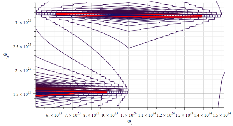
Mass levels graph showing the “standard” value of mass for the Aluminum atomic nucleus

The estimated parameters and amplitude values in Fig. 15 are:

$r_n={3.5\ 10}^{-15}\left[m\right]$

$A_e={3.5\ 10}^{-17}\left[m\right]$

$A_p={10}^{-3}A_e\left[m\right]$

The exact “standard” mass value is in the region marked by the two red contours (or level lines): $m={4.48\ 10}^{-26}\left[Kg\right]$

The electron central frequencies range approximately from $f_{e1}\cong8\ {10}^{22}\ [Hz]$ to $f_{e2}\cong1.6\ {10}^{23}\ [Hz]$ , while the proton central frequencies vary from approximately $f_{p1}\cong2.4\ {10}^{24}\ [Hz]$ to $f_{p2}\cong5.1\ {10}^{25}\ [Hz]$ .

Figure 16
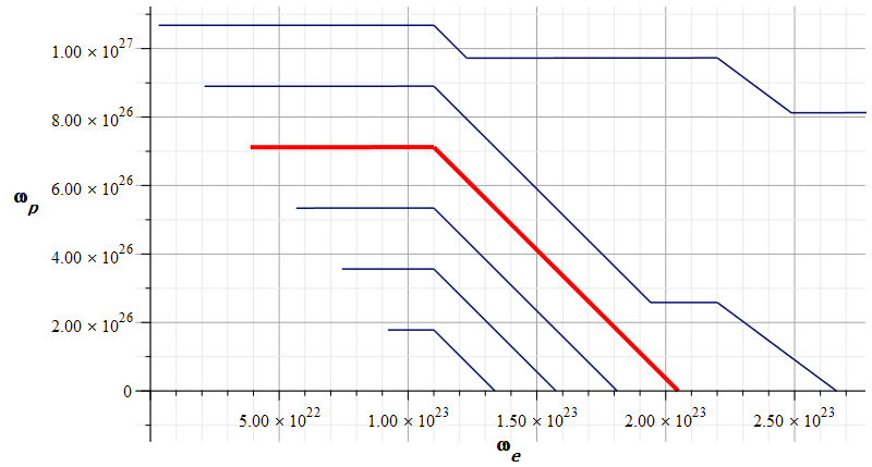
Mass levels graph showing the “standard” value of mass for the Aluminum atomic nucleus, by changing the parameters used in Fig. 15

The estimated parameters and amplitude values in Fig. 16 are:

$r_n={3.5\ 10}^{-15}\left[m\right]$

$A_e={1.71\ 10}^{-17}\left[m\right]$

$A_p={10}^{-3}A_e\left[m\right]$

The exact “standard” mass value is in the region marked by the three red contours (or level lines): $m={4.48\ 10}^{-26}\left[Kg\right]$

The electron central frequencies range approximately from $f_{e1}\cong9\ {10}^{22}\ [Hz]$ to $f_{e3}\cong1.6\ {10}^{23}\ [Hz]$ , while the proton central frequencies vary from approximately $f_{p1}\cong2.8\ {10}^{24}\ [Hz]$ to $f_{p3}\cong8\ {10}^{25}\ [Hz]$ .

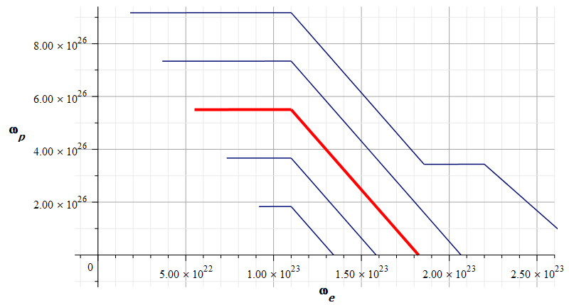
The following images show very approximate values of the “standard” mass of the Aluminum nucleus, according to the different values of parameters and variables.

Figure 17
Mass levels graph showing approximate value of mass for the Aluminum atomic nucleus

The estimated parameters and amplitude values in Fig.17 are:

$r_n={3.5\ 10}^{-15}\left[m\right]$

$A_e={0.4\ 10}^{-16}\left[m\right]$

$A_p={10}^{-3}A_e\left[m\right]$

The approximate “standard” mass value is in the region marked by the red contour line (or level line): $m={4.52\ 10}^{-26}\left[Kg\right]$

The electron central frequency is approximately $f_e\cong2.4\ {10}^{22}\ [Hz]$ , while the proton central frequency is approximately $f_p\cong6.3\ {10}^{25}\ [Hz]$ .

Figure 18
Mass levels graph showing approximate value of mass for the Aluminum atomic nucleus, by changing the parameters used in Fig. 17

The estimated parameters and amplitude values in Fig. 18 are:

$r_n={2.4\ 10}^{-15}\left[m\right]$

$A_e={0.9\ 10}^{-16}\left[m\right]$

$A_p=\frac{{10}^{-3}}{3}A_e\left[m\right]$

The approximate “standard” mass value is in the region marked by the red contour line (or level line): $m={4.64\ 10}^{-26}\left[Kg\right]$

The electron and proton central frequencies are approximately the same as those in Fig. 17.

Figure 19
Mass levels graph showing approximate value of mass for the Aluminum atomic nucleus, by changing the parameters used in Fig. 17 and Fig. 18

The estimated parameters and amplitude values in Fig. 18 are:

$r_n={7.97\ 10}^{-13}\left[m\right]$

$A_e={\ 10}^{-13}\left[m\right]$

$A_p=\frac{A_e}{10}\left[m\right]$

The approximate “standard” mass value is in the region marked by the red contour lines (or level lines): $m={4.51\ 10}^{-26}\left[Kg\right]$

The lowest-average electron and proton frequencies are approximately in the range of $f\cong1.6\ {10}^{16}\ [Hz]$ . For this particular case, the lowest electron frequency is $f=0\ [Hz]$ (first red contour line around the origin).

Note that in the preceding cases, the proton and electron oscillation frequencies lie between Visible/Near UV to the range of gamma radiation.

The atomic model described in previous paragraphs predicts a high elasticity of the particles, which yields a drastic change in size. Therefore, the estimated nucleus size and amplitude of oscillations might adopt values such that the proton and electron frequencies may greatly differ from the values shown above. Based on pure estimations, we may expect to deal with a radiation spectrum probably ranging from microwaves to gamma radiation.

This situation will last until experiments determine realistic values.

A nuclear wave equation is derived in Part-2, which will give a better insight into nuclear radiation frequencies.

Conclusions

It has been demonstrated that mass is not a fundamental quantity, but an intrinsic property of atoms, which arises from the electrodynamic interaction of the elementary particles in the nucleus. Its value is constant only for the “natural state” of oscillation of the atomic nucleus shells.

By applying the universal force to a contemporary model of atomic structure, it was demonstrated that the mass value depends on the oscillation of electron and proton shells in the nucleus. The mass magnitude and sign might be changed at will by external agents.

Analysis in the time and frequency domains have revealed the regions of positive and negative mass. A Fourier analysis clearly shows the main frequency and the harmonics, while the phase swings between $\pm\pi$ demonstrate a succession of resonance states.

The “standard” mass of the Aluminum atom was obtained through several examples by using the intrinsic mass formula.

Bibliography

[1]. Shanshan Yao, Xiaoming Zhou and Gengkai Hu, “Experimental study on negative effective mass in a 1D mass–spring system” (2008), New Journal of Physics (2008). https://iopscience.iop.org/article/10.1088/1367-2630/10/4/043020/pdf

[2]. J. P. Wesley, “Inertial Mass of a Charge in a Uniform Electrostatic Potential Field” (2001), Annales Foundation Louis de Broglie, Volume 26, nr. 4 (2001).

[3]. V. F. Mikhailov, “Influence of an electrostatic potential on the inertial electron mass” (2001), Annales Foundation Louis de Broglie, Volume 26, nr. 4 (2001).

[4]. M. Weikert and M. Tajmar, “Investigation of the Influence of a field-free electrostatic Potential on the Electron Mass with Barkhausen-Kurz Oscillation” (2019), ), Annales Foundation Louis de Broglie, Volume 44, (2019).

[5]. Timothy H. Boyer, “Electrostatic potential energy leading to a gravitational mass change for a system of two point charges” (1979), American Journal of Physics 47, 129 (1979), https://aapt.scitation.org/doi/10.1119/1.11881

[6]. A. K. T. Assis, “Changing the Inertial Mass of a Charged Particle” (1992), Journal of the Physical Society of Japan Vol. 62, No. 5, May, 1993, pp. 1418-142, https://journals.jps.jp/doi/abs/10.1143/JPSJ.62.1418?journalCode=jpsj

[7]. M. Tajmar, “Propellantless propulsion with negative matter generated by electric charges” (2013), Technische Universität Dresden (2013), https://tu-dresden.de/ing/maschinenwesen/ilr/rfs/ressourcen/dateien/forschung/folder-2007-08-21-5231434330/ag_raumfahrtantriebe/JPC—Propellantless-Propulsion-with-Negative-Matter-Generated-by-Electric-Charges.pdf?lang=en

[8]. M. Tajmar and A. K. T. Assis, “Particles with Negative Mass: Production, Properties and Applications for Nuclear Fusion and Self-Acceleration” (2015), https://www.ifi.unicamp.br/~assis/J-Advanced-Phys-V4-p77-82(2015).pdf

[9]. M. A. Khamehchi, Khalid Hossain, M. E. Mossman, Yongping Zhang, Th. Busch, Michael McNeil Forbes, and P. Engels, “Negative-Mass Hydrodynamics in a Spin-Orbit–Coupled Bose-Einstein Condensate” (2017), Phys. Rev. Lett. 118, 155301 (2017), https://journals.aps.org/prl/abstract/10.1103/PhysRevLett.118.155301

[10]. David L. Bergman, J. Paul Wesley, “Spinning Charged Ring Model of Electron Yielding Anomalous Magnetic Moment” (1990).

[11]. Joseph Lucas and Charles W. Lucas, Jr., “A Physical Model for Atoms and Nuclei”, Galilean Electrodynamics, Volume 7, Number 1 (1996), Foundations of Science (2002-2003), Part 1, Part 2, Part 3, Part 4.

[12]. Charles W. Lucas, Jr., “Derivation of the Universal Force Law”, Foundations of Science (2006-2007), Part 1, Part 2, Part 3, Part 4.

[13]. Arthur H. Compton, “The size and shape of the electron” (1918), Journal of the Washington Academy of Sciences, Vol. 8, No. 1, https://www.jstor.org/stable/24521544

[14]. David L. Bergman, “Modeling the Real Structure of an Electron” (2010), Foundations of Science.

[15]. David L. Bergman, “Shape & Size of Electron, Proton & Neutron” (2004), Foundations of Science.

[16]. Zoran Jaksic, N. Dalarsson, Milan Maksimovic, “Negative Refractive Index Metamaterials: Principles and Applications” (2006), https://www.researchgate.net/publication/200162674_Negative_Refractive_Index_Metamaterials_Principles_and_Applications

Negative Mass and Negative Refractive Index in Atom Nuclei – Nuclear Wave Equation – Gravitational and Inertial Control <Part-2>

Negative Mass and Negative Refractive Index in Atom Nuclei – Nuclear Wave Equation – Gravitational and Inertial Control <Part-3>

Negative Mass and Negative Refractive Index in Atom Nuclei – Nuclear Wave Equation – Gravitational and Inertial Control <Part-4>

Negative Mass and Negative Refractive Index in Atom Nuclei – Nuclear Wave Equation – Gravitational and Inertial Control <Part-5>

Negative Mass and Negative Refractive Index in Atom Nuclei – Nuclear Wave Equation – Gravitational and Inertial Control <Part-6>

What is Charge? – The Redefinition of Atom – Energy to Matter Conversion

Physics Answers

Negative Mass and Negative Refractive Index in Atom Nuclei – Nuclear Wave Equation – Gravitational and Inertial Control
-(Part 1)-

Abstract

Introduction

The Universal Force Law

A Connected Universe under Continuous Radiation

Forces in Atom Nuclei

Coulomb Force Among Nuclear Shells

Averaging the distance between two shells