Raul Fattore
March 20, 2022
Table of Contents
Abstract
The causes of dynamic deformation of the Earth and motion effects induced by the universe’s gravitational field and from neighboring celestial bodies are easily explained in the present study.
- Is the deformation of the Earth static, dynamic, or both?
- Is the gravitational field the only cause of the deformation of the Earth?
- How do the masses of near celestial bodies impact locally?
- Does the mass of the universe contribute to local effects in order to be considered?
- How is the Earth’s orbit modified by this force interchange?
In this analysis, there are several cases that show with clarity what accelerations produce what effect and in what amount. The differential equations of a force in space are derived for those of you who want to make heavy calculations (see APPENDIX).
Introduction
The first law of Newton states: “A body continues in its state of rest, or in uniform motion in a straight line, unless acted upon by a force.”
A body can be considered “at rest” or moving in a straight line at constant velocity if the sum of accelerations (forces) acting on it is equal to zero. But these conditions will not always apply, depending on what frame of reference we take.
If we are traveling in a car in a straight line at a constant velocity of 100 Km/h, we are “at rest” (acceleration = 0 m/s2) with respect to the car, or we are moving at 100 Km/h (acceleration = 0 m/s2) with respect to some fixed point of reference on an ideal non-spinning Earth. The first Newton’s law is apparently valid in such a case. Whether we chose the car, the passenger, or a fixed point, in all these cases our reference is called an inertial frame of reference because no accelerations are present.
However, if the car is taking a curve without sliding, it is subject to a centripetal acceleration that points to the center of curvature. Since we move free inside the car because we are not tied with any mean to the center of curvature, then we feel the opposite acceleration called centrifugal acceleration, which pulls us to the exterior of the curve. In this case, the first law of Newton is not applicable to both reference frames (car and passenger), which now are called non-inertial frames of reference because the motion is subject to accelerations.
The States of “Rest” and Uniform “Rectilinear” Motion Don’t Exist in the Universe
If we take the center of mass of the Earth as the origin of a rotating frame of reference, then the first law of Newton cannot be applied. The same happens if we take the center of mass of the solar system or that of the Universe as our frame of reference.
In the example of the car above, even if we take the vehicle as our reference system, we are not “at rest” inside the car. As a passenger, we are also subject to the gravitational and centrifugal accelerations of Earth, and the gravitational acceleration produced by the distribution of mass in the Universe (our solar system plus the rest of the galaxies in the visible Universe). So, when we say that we are “at rest” with respect to the car, we are simply ignoring the laws of Mother Nature.
Therefore, the states of “rest” and that of a uniform “rectilinear” motion do not exist in the universe.
However, the first law of Newton helps us to predict the motion of bodies with good approximation in several cases.
Considering The “Mach’s Principle”
Objects in the Universe are subject to the continued actions of forces (accelerations) because of rotation, translation, electromagnetic, and gravitational interactions with nearby and distant surrounding bodies.
Under many circumstances, we may neglect external accelerations because they might be of low magnitude compared to local accelerations. But that doesn’t mean that they don’t exist. Moreover, subtle differences in acceleration are the cause of constant and dynamic deformation of masses and changes in motion that can’t be ignored.
How the Amount of Mass of the Universe Changes With Distance
If we assume that our visible Universe is spherical, with a homogeneous density of mass in all directions (isotropic), then the change in mass with respect to a change in volume will be given by:
dm=\rho_udV (a)
Let’s consider two concentric spheres as in the figure. The volume change is given by:
dV=\frac{4}{3}\pi\left(r+dr\right)^3-\frac{4}{3}\ \pi\ r^3,
dV=\frac{4}{3}\pi\left(r^3+3r^2dr+3r{\rm dr}^2+{\rm dr}^3-r^3\right)
When neglecting the higher-order terms in dr and simplifying, we get:
dV\cong4\ \pi{\ r}^2\ dr (b)
By replacing (b) in (a), we obtain:
| dm=\rho_u4\ \pi\ r^2dr | => | \frac{dm}{dr}=\rho_u4\ \pi\ r^2 |
We see that the amount of mass increases with the square of the distance.
Mass and Radius of the Visible Universe
The estimated values of the mass and radius are:
| M_u\cong1.5\ {10}^{53}\ Kg (d) | With an approximate density: | \rho_u\cong{10}^{-29}\ \frac{Kg}{m^3} (e) |
r_u\cong9\ {10}^{26}\ m (f) |
Effects on Earth Caused By Local Accelerations
The rotation of the Earth on its axis added to its own gravity acceleration are both the cause of a constant (permanent) deformation of the planet. In the next paragraphs, we’ll see that, besides the constant deformation, there is also a dynamic deformation that will affect the shape of the Earth as well as induce additional motions to rotation and translation.
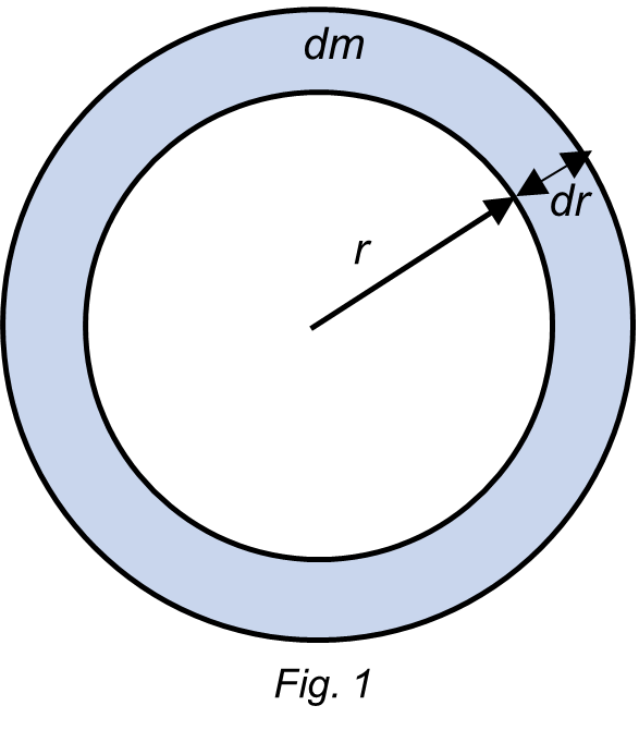
Let’s take a spherical shell of mass dm and thickness dr on the surface of the Earth.
The gravitational acceleration caused by the Earth on the shell is denoted as a_E.
Since the Earth is spinning at an angular velocity \dot{\emptyset}, the shell is also under the action of a centripetal acceleration:
{-a}_c=R{\dot{\emptyset}}^2 (1)
This acceleration is equal in magnitude and opposite to the centrifugal acceleration a_f.
But the distance R depends on the polar angle \theta:
R=r\sin{\theta} (2)
By replacing (2) in (1), we get:
-a_c=a_f=rsin{\theta}{\dot{\emptyset}}^2 (3)
The centripetal/centrifugal acceleration is maximum at the equator and vanishes at the poles.
The maximum value of the centrifugal acceleration is: a_f=6.4\ {10}^6\ \left(7.27\ {10}^{-5}\right)^2=3.38\ {10}^{-2}\ \frac{m}{s^2} (4)
Based on spatial spherical coordinates (see APPENDIX), and since the Earth rotates at constant angular velocity \dot{\emptyset}, the component of the acceleration in the \hat{\emptyset} direction is zero. Therefore, the centrifugal acceleration reduces to two components, one in the direction of the Earth’s radius a_{cr}, and the other in the polar direction a_{c\theta}. That is,
a_f=a_{cr}\hat{r}+a_{c\theta}\hat{\theta}+0\hat{\emptyset} (5)
The projection of the centrifugal acceleration a_f on the Earth’s gravitational acceleration (a_E) line is:
a_{cr}=a_f\cos{\left(\frac{\pi}{2}-\theta\right)}=a_f\sin{\theta} (6)
By replacing (3) in (6):
a_{cr}=r\ {sin}^2\left(\theta\right)\ {\dot{\emptyset}}^2 (7)
The acceleration component in the polar direction is:
| a_{c\theta}=a_f\sin{\left(\frac{\pi}{2}-\theta\right)}=a_f\cos{\theta} | => | a_{c\theta}=r\sin{\theta}\cos{\theta}{\dot{\emptyset}}^2 (8) |
By replacing (7) and (8) in (5),
a_f=r\ {sin}^2\left(\theta\right)\ {\dot{\emptyset}}^2\ \hat{r}+r\sin{\theta\cos{\theta}}{\dot{\emptyset}}^2\hat{\theta}
The component that directly affects the Earth’s gravity is a_{cr}, which is opposite to a_E. The resultant acceleration is a modified Earth’s gravity acceleration, which is a function of the polar angle and is the local cause of Earth’s deformation.
Constant Deformation of Earth Caused by Local Accelerations – Rigidity of a Mass
The rigidity of a mass is determined by the amount of deformation of the mass’ shape under the action of a force. A “rigid body” is just an idealization because there will always be some amount of deformation when a mass is under the action of a force, even when we are not able to measure it. As a rough approximation, we can say that solids are “more rigid” than liquid or gases because fluids don’t have the ability to resist deformation.
The Earth is composed of a vast variety of solid materials. as well as liquids and gases. Therefore, it is not exempt from deformations under the actions of accelerations.
Particles in the shell of Fig. 2 can be more or less rigid, and they will have the same experience as the passenger inside the car which is taking a curve. Those particles will be pushed away from the center of curvature because of the centrifugal force a_f. The “less rigid” matter (gas, liquid) will stretch more than solid materials (minerals).
The local resultant acceleration on every piece of mass in the shell of Fig. 2 is:
| a_{res}={-a}_E+a_{cr} | => | a_{res}={-a}_E+r\ {sin}^2\left(\theta\right){\dot{\emptyset}}^2 (10) |
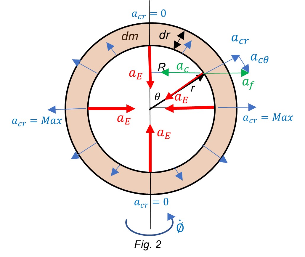
This acceleration is maximum at the poles: a_{res}=-a_E+0=-9.8\ \frac{m}{s^2}, and has its minimum magnitude at the equator (see Eq. 10):
a_{res}={-a}_E+r\ {\dot{\emptyset}}^2=-9.8+3.38\ {10}^{-2}=-9.766\ \frac{m}{s^2}
The “compression” caused by the acceleration on the poles and the “expansion” produced by the lower acceleration on the equator make a constant deformation of the Earth. As a result, there is a little flattening on the poles, as shown with exaggeration in Fig. 3.
This phenomenon is characteristic of any spinning body.
If the angular velocity of the Earth were high enough such that the centrifugal force is comparable to the gravitational acceleration, then the Earth will start breaking apart.
Dynamic Deformation of Earth and Motion Effects due to Gravitational Accelerations from the Universe and Near Celestial Bodies
There are two types of dynamic effects:
- Dynamic deformation of mass
- Dynamic change in motion
As we have seen in previous paragraphs, the local accelerations on Earth are the cause of the constant deformation of the planet. However, it is hard to imagine that any celestial body is shielded from external accelerations caused by other celestial bodies.
The fact that all bodies in the universe move relative to each other will change the magnitude of accelerations among them with time, causing thus dynamic deformations on the bodies as well as a sort of combined motions.
1. Dynamic deformation of mass
In this paragraph, we are going to analyze how the external accelerations add a dynamic deformation to the Earth and a dynamic change in motion. The analysis of the relative motion between two celestial bodies is treated in another paper.
When external forces (accelerations) are acting on the shell of Fig. 2, the resultant acceleration will have three spatial components in spherical coordinates (see motion in spherical coordinates and components of a force in space).
Regardless of the direction of the external accelerations, there will always be a radial component that can point in one direction or another, depending on the location of the celestial bodies. The radial component for accelerations at polar angles \theta\neq0^{\circ} and \theta\neq180^{\circ} is given by:
a_r=a\sin{\theta} (11)
Equation (11) is not applicable when the external acceleration is aligned with one of the poles, where \theta=0^{\circ} or \theta=180^{\circ}. In this case:
a_r=a
This acceleration which is caused by distant celestial bodies changes with time, having its maximum at the equator and vanishing at the poles (except when it is aligned with the poles). It causes a dynamic deformation of the Earth that is added to the permanent (constant) deformation analyzed in the previous paragraph.
2. Dynamic change in motion
Celestial bodies move freely in space and are under the action of their own accelerations as well as those from distant bodies. So far, we have analyzed the external acceleration on both sides of a spherical shell to see the extent of deformation in function of the resultant acceleration at both sides of the shell. However, a motion analysis requires that we study the resultant acceleration at the center of mass of the body.
Perhaps the most important effect of external accelerations acting on any celestial body is not its subtle change in shape, but the induced change in motion. Let’s roughly consider the motion effects on the Earth caused by the Sun and the Moon.
| \mathbf{a}_\mathbf{E}=9.8\ [\frac{m}{s^2}] Earth’s gravity acceleration | \mathbf{a}_{\mathbf{ES}}=1.75\ {10}^{-8}\ \left[\frac{m}{s^2}\right]\ Earth’s gravity acceleration on the Sun | |
| \mathbf{a}_\mathbf{S}=5.9\ {10}^{-3}\ \left[\frac{m}{s^2}\right]\ Sun’s gravity acceleration on the Earth | \mathbf{a}_{\mathbf{EM}}=2.67\ {10}^{-3}\ \left[\frac{m}{s^2}\right]\ Earth’s gravity acceleration on the Moon | |
| \mathbf{a}_\mathbf{M}=3.3\ {10}^{-5}\ \left[\frac{m}{s^2}\right]\ Moon’s gravity acceleration on the Earth |
Note:
It’s nonsense to consider the Earth’s dimensions for a good reason: the distances Earth-Sun and Earth-Moon change between 476 and 3.3 times the Earth’s diameter, respectively.
a. Sun and Moon on each side of the Earth.
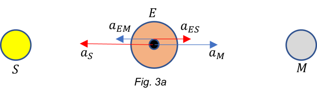
Taking the Earth as a reference, and considering the action-reaction pairs, the resultant acceleration is:
a_{res}=-a_S+a_{ES}+a_M-a_{EM}=-5.9\ {10}^{-3}+1.75\ {10}^{-8}+3.3\ {10}^{-5}-2.67\ {10}^{-3}=-8.53\ {10}^{-3}\ [\frac{m}{s^2}] (11a)
b. Sun and Moon on the same side of the Earth.
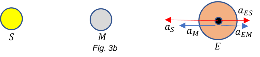
Taking the Earth as a reference, and considering the action-reaction pairs, the resultant acceleration is:
a_{res}=-a_S+a_{ES}-a_M+a_{EM}=-5.9\ {10}^{-3}+1.75\ {10}^{-8}-3.3\ {10}^{-5}+2.67\ {10}^{-3}=-3.26\ {10}^{-3}\ [\frac{m}{s^2}] (11b)
The Earth’s translation motion is not elliptical
The Earth revolves around the sun with a centripetal acceleration equal to the gravitational acceleration of the sun on Earth, that is a_S=-5.9\ {10}^{-3}\ \left[\frac{m}{s^2}\right]. However, this is not a constant value as we can see from (11a) and (11b), which gives \Delta a_{res}=-8.53\ 10^{-3}-(-3.26\ 10^{-3})=-5.27\ 10^{-3} [\frac{m}{s^{2}}], with a mean value of \frac{\Delta a_{res}}{2}=-2.63\ 10^{-3} [\frac{m}{s^{2}}]. Then, the maximum changes in acceleration are:
a=-5.9\ {10}^{-3}\ \pm2.63\ {10}^{-3}\ \left[\frac{m}{s^2}\right]]
The resultant acceleration oscillates between the maximum values as the Moon revolves around the Earth, with a period of 27.3 days (one revolution of the Moon around Earth).
The above results tell us that the Earth is revolving around the Sun not by following an elliptic line but oscillating around the mean value of an elliptical line as shown exaggerated in Fig. 3c. The orbit trajectory is modulated by a periodic function. There are ~ 13 periods in one revolution.

Note that a change in acceleration with time, which is known as jerk, is the source of an oscillatory motion that can be periodic with a fixed or variable frequency. Though I’m not going to dig into this effect, the definition of jerk is: \vec{j}=\frac{d\vec{a}}{dt}\ [\frac{m}{s^3}].
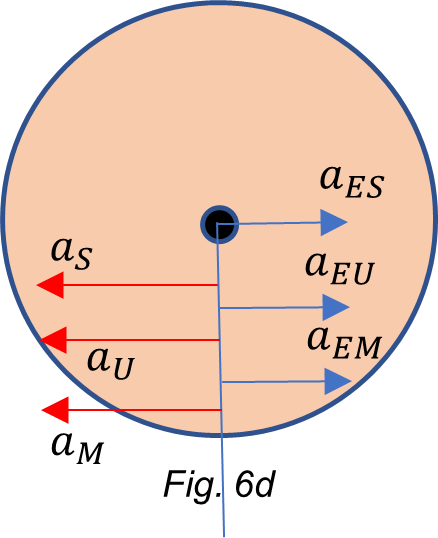
Case 1: Sun and Moon aligned at opposite faces of the Earth; center of mass of the Universe aligned on Moon’s side.
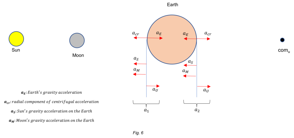
For simplicity, let’s consider the accelerations at the Earth’s equator caused by the neighbor and distant celestial bodies on a thin spherical shell, as shown in Fig. 4. Let’s assume that the effect of the shell mass is negligible on the other bodies. Overlapping all accelerations in the equatorial line will be confusing, so to identify each one, let distribute them in vertical lines at both sides of the Earth for easy recognition. The center of mass of the Universe is denoted as “comu”.
Note:
It’s nonsense to consider the Earth’s dimensions for a good reason: the distances Earth-Sun and Earth-Moon change between 476 and 3.3 times the Earth’s diameter, respectively.
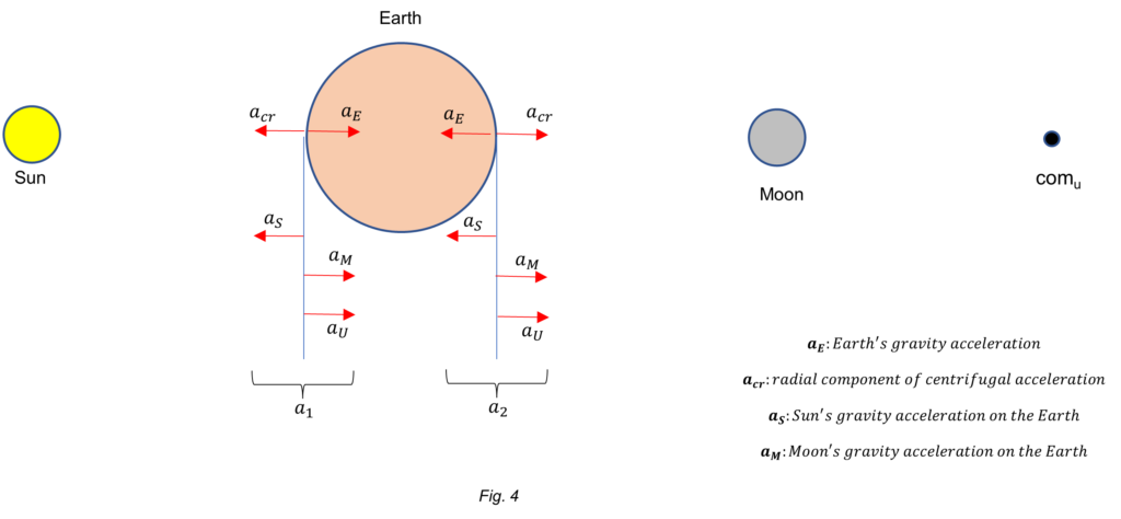
Let’s define the sum of accelerations at each side of the Earth as a_1 and a_2:
a_1=a_E+a_M+a_U-a_S-a_{cr}
a_2=a_{cr}+a_M+a_U-a_S-a_E
As we have seen in previous paragraphs, the estimated values of the mass and radius of the Universe are:
| M_u\cong1.5\ {10}^{53}\ Kg | and | r_u\cong9\ {10}^{26}\ m |
We ignore where the Earth is located with respect to the center of mass of the Universe (comu) and at what distance. If we assume that the Earth is at a distance r={10}^{23}\ m of comu, then the gravitational acceleration on Earth caused by the universal mass will be: a_U=\frac{GM_U}{r^2}={10}^{-3}\ [\frac{m}{s^2}]. Then, the magnitude of all the accelerations on Earth are:
| a_U={10}^{-3}\ [\frac{m}{s^2}]; | a_E=9.8\ [\frac{m}{s^2}]; | a_M=3.3\ {10}^{-5}\ [\frac{m}{s^2}]; | a_S=5.9\ {10}^{-3}\ [\frac{m}{s^2}]; | a_{cr}=3.3\ {10}^{-2}\ [\frac{m}{s^2}] |
By plugging these values in a_1 and a_2 above, we obtain the magnitude of the accelerations at both faces of the Earth:
a_1=9.8+3.3\ {10}^{-5}+{10}^{-3}-5.9\ {10}^{-3}-3.3\ {10}^{-2}=9.7621\ [\frac{m}{s^2}] (12)
a_2=3.3\ {10}^{-2}+3.3\ {10}^{-5}+{10}^{-3}-5.9\ {10}^{-3}-9.8=-9.7718\ [\frac{m}{s^2}] (13)
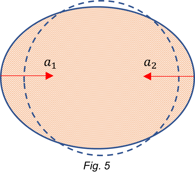
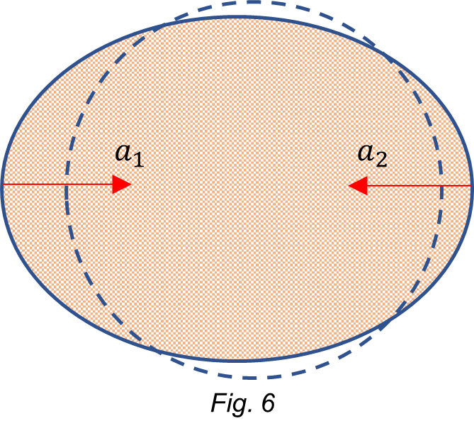
We see that the dynamic resultant of the gravitational acceleration on Earth’s surface is weaker on the Sun’s side, causing thus a bigger dynamic “stretching” than that on the Moon’s side, as shown in Fig. 5.
Recall that the magnitudes of both accelerations increase when approaching the poles.
Out of the Earth’s gravitational acceleration, the radial components of all other accelerations decrease away from the equator until vanishing at the poles according to Eq. (11). At the poles:
| a_1=9.8\ [\frac{m}{s^2}] | and | a_2=-9.8\ [\frac{m}{s^2}] |
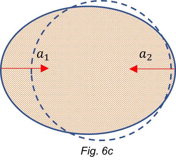
Case 2: Sun and Moon aligned both with one face of the Earth; center of mass of the Universe aligned with the opposite Earth’s face.
For simplicity, let’s consider the accelerations at the Earth’s equator caused by the neighbor and distant celestial bodies on a thin spherical shell, as shown in Fig. 6. Let’s assume that the effect of the shell mass is negligible on the other bodies. Overlapping all accelerations in the equatorial line will be confusing, so to identify each one, let distribute them in vertical lines at both sides of the Earth for easy recognition. The center of mass of the Universe is denoted as “comu”.
Note:
It’s nonsense to consider the Earth’s dimensions for a good reason: the distances Earth-Sun and Earth-Moon change between 476 and 3.3 times the Earth’s diameter, respectively.
In this case, the sum of accelerations at each side of the Earth are:
a_1=a_E+a_U-a_{cr}-a_S-a_M
a_2=a_{cr}+a_U-a_E-a_S-a_M
By plugging the values of the accelerations in a_1 and a_2 above, we obtain the magnitude of the accelerations at both faces of the Earth:
a_1=9.8+{10}^{-3}-3.3\ {10}^{-2}-5.9\ {10}^{-3}-3.3\ {10}^{-5}=9.7620\ [\frac{m}{s^2}]
a_2=3.3\ {10}^{-2}+{10}^{-3}-9.8-5.9\ {10}^{-3}-3.3\ {10}^{-5}=-9.7719\ [\frac{m}{s^2}]
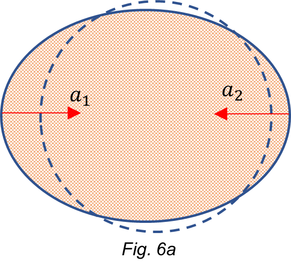
There is just a subtle difference to be appreciated with respect to Case 1.
Here, again, the dynamic resultant of the gravitational acceleration on Earth’s surface is weaker on the Sun-Moon side, causing thus a bigger dynamic “stretching” than that on the “comu” side, as shown in Fig. 6. Note that the stretching on the Sun-Moon side is a little bit more than in the previous case.
Recall that the magnitudes of both accelerations increase when approaching the poles.
Out of the Earth’s gravitational acceleration, the radial components of all other accelerations are decreasing away from the equator until vanishing at the poles according to Eq. (11).
At the poles: a_1=9.8\ [\frac{m}{s^2}] and a_2=-9.8\ [\frac{m}{s^2}].
What happens when the Center of Mass of the Universe (comu) is at the opposite side of the Earth in Fig. 4 and Fig. 6
Regarding deformation, the resultant accelerations from Fig. 4 will be:
a_1=a_E+a_M-a_U-a_S-a_{cr}
a_2=a_{cr}+a_M-a_U-a_S-a_E
By replacing values, we get:
a_1=9.8+3.3\ {10}^{-5}-{10}^{-3}-5.9\ {10}^{-3}-3.3\ {10}^{-2}=9.7601\ [\frac{m}{s^2}] (16)
a_2=3.3\ {10}^{-2}+3.3\ {10}^{-5}-{10}^{-3}-5.9\ {10}^{-3}-9.8=-9.7738\ [\frac{m}{s^2}] (17)
By comparing (12) with (16) and (13) with (17), we see an even weaker acceleration on the left side and stronger on the right side of the Earth. The deformation is stronger than that in Fig. 4.
Regarding motion, taking the Earth as a reference and considering the action-reaction pairs, the resultant acceleration is:
a_{res}={-a}S+a{ES}-a_U+a_{EU}+a_M-a_{EM}=-5.9\ {10}^{-3}+1.75\ {10}^{-8}-{10}^{-3}+3.9\ {10}^{-32}+3.3\ {10}^{-5}-2.67\ {10}^{-3}=-9.53\ {10}^{-3}\ [\frac{m}{s^2}]
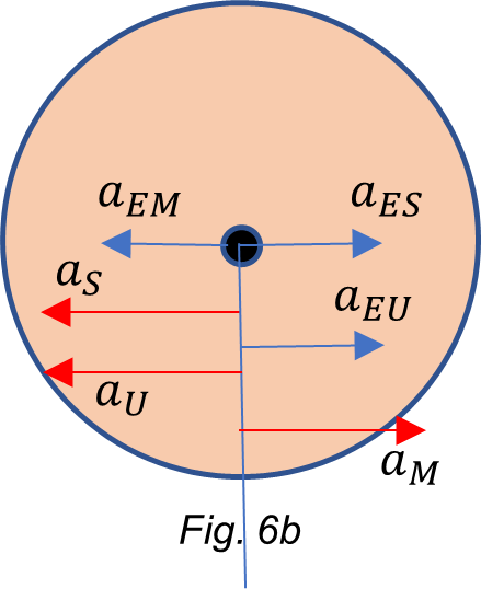
a_{EU}:Earth\ gravity\ acceleration\ on\ the\ Universe\ center\ of\ mass
The resultant acceleration is higher than that of the Sun on Earth and points to the Sun and the Universe’s center of mass. It could easily be a centripetal acceleration that makes the Earth and the whole solar system or even the Milky Way orbit around comu.
Regarding deformation, the resultant accelerations from Fig. 6 will be:
a_1=a_E-a_U-a_{cr}-a_S-a_M
a_2=a_{cr}-a_U-a_E-a_S-a_M
By replacing values, we get:
a_1=9.8-{10}^{-3}-3.3\ {10}^{-2}-5.9\ {10}^{-3}-3.3\ {10}^{-5}=9.7600\ [\frac{m}{s^2}] (18)
a_2=3.3\ {10}^{-2}-{10}^{-3}-9.8-5.9\ {10}^{-3}-3.3\ {10}^{-5}=-9.7739\ [\frac{m}{s^2}] (19)
By comparing (14) with (18) and (15) with (19), we see a further decrease in acceleration on the left side and a further increase in acceleration on the right side of the Earth. The deformation is the strongest.
Regarding motion, taking the Earth as a reference and considering the action-reaction pairs, the resultant acceleration is:
a_{res}={-a}_S+a_{ES}-a_U+a_{EU}-a_M+a_{EM}=-5.9\ {10}^{-3}+1.75\ {10}^{-8}-{10}^{-3}+3.9\ {10}^{-32}-3.3\ {10}^{-5}+2.67\ {10}^{-3}=-4.26\ {10}^{-3}\ [\frac{m}{s^2}]
Though counter-intuitive, the resultant acceleration is less than that calculated for Fig. 4 and points to the Sun and the Universe’s center of mass. It could easily be a centripetal acceleration that makes the Earth and the whole solar system or even the Milky Way orbit around comu.
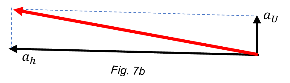
What happens when the Center of Mass of the Universe (comu) is aligned with one pole in Fig. 4 and Fig. 6
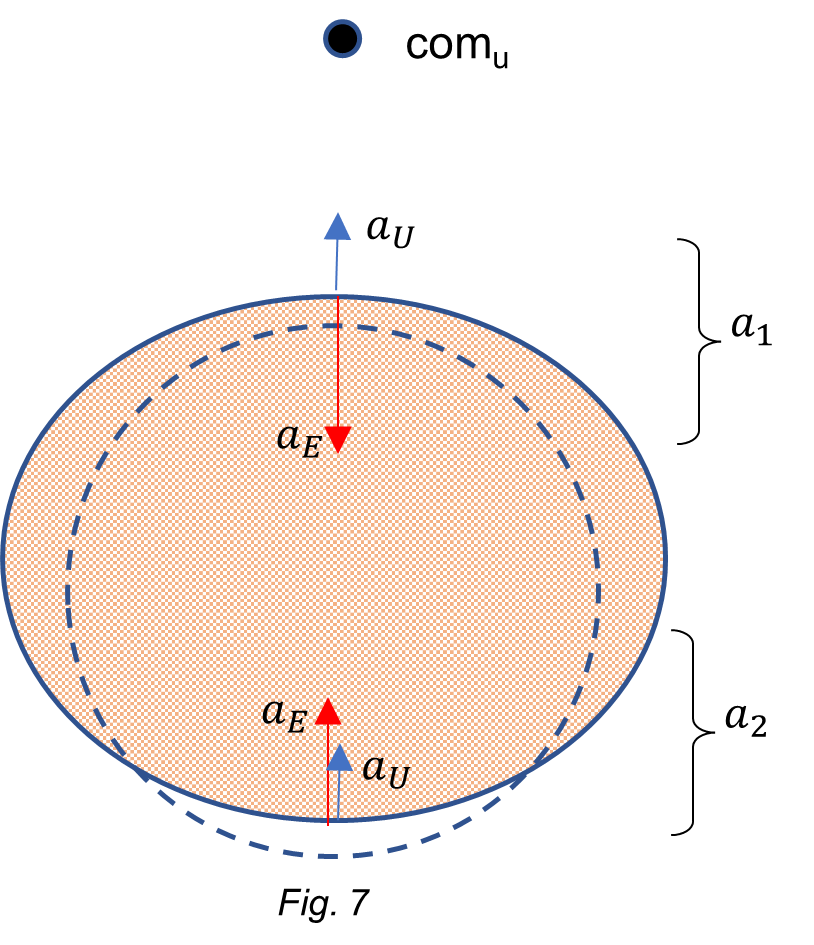
In this case, the acceleration caused by the center of mass of the Universe is perpendicular to the accelerations parallel to the equator and perpendicular to the Earth’s plane of rotation. So, it’s easy to see that the deformation effect of a_U will be a “stretching” along the polar axis or rotation axis of the Earth.
Regarding deformation, let’s define a_1 as the resultant acceleration on the comu side, and a_2 the resultant acceleration on the opposite pole:
a_1=a_U-a_E={10}^{-3}-9.8=-9.799\ [\frac{m}{s^2}]
a_2=a_E+a_U=9.8+{10}^{-3}=9.801\ [\frac{m}{s^2}]
The upper resultant acceleration is weaker than the lower one, causing thus a stretching of the upper pole toward comu. The resultant acceleration in the lower pole is higher than the gravitational acceleration of the Earth, causing a “compression” toward comu.
Regarding motion, taking the Earth as a reference and considering the action-reaction pairs, the resultant acceleration is:
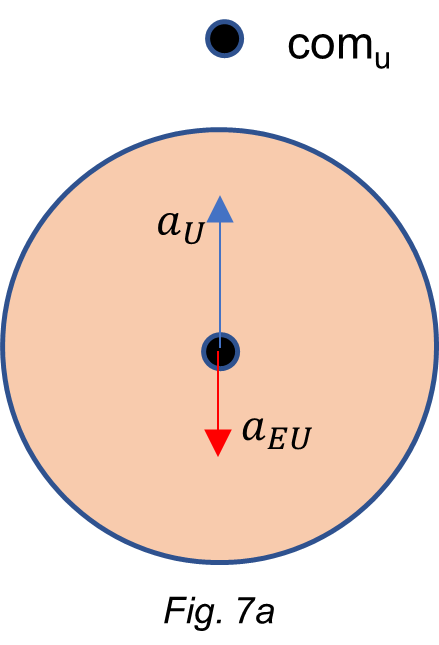
a_{res}=a_U-a_{EU}={10}^{-3}-3.9\ {10}^{-32}\cong{10}^{-3}\ [\frac{m}{s^2}]
This acceleration is considerable and points to the Universe’s center of mass.
The addition of this acceleration to the horizontal resultant acceleration caused by the Sun-Moon will constitute the final resultant.
If Sun and Moon are both on the same side of the Earth, the horizontal resultant is:
a_h={a_S+a}_M=5.9\ {10}^{-3}+3.3\ {10}^{-5}=5.933\ {10}^{-3}\ [\frac{m}{s^2}]
The final resultant acceleration pulls a bit the Earth in the direction of comu perhaps causing a shift of the Earth’s orbit plane around the sun.
There is a subtle difference in the result when Sun and Moon are each on both sides of the Earth.
The Importance of the Universe Mass
The results obtained with Eq. (16) to (19) have significant importance when compared with those of Eq. (12) to (15). The change in the magnitude of the resultant accelerations cannot be disregarded when we consider the effects on Earth of the gravitational accelerations of distant galaxies or that of the Universe’s center of mass.
By taking the situation in Fig. 4, we have the following acceleration differences when the position of comu is at the opposite side of the Earth:
\Delta a_{1}=(12)-(16)=9.7621-9.7601=2\ 10^{-3} [\frac{m}{s^{2}}]
\Delta a_{2}=(13)-(17)=-9.7718+9.7738=2\ 10^{-3} [\frac{m}{s^{2}}]
By taking the situation in Fig. 6, we have the same acceleration differences when the position of comu is at the opposite side of the Earth:
\Delta a_{1}=(14)-(18)=9.7620-9.7600=2\ 10^{-3} [\frac{m}{s^{2}}]
\Delta a_{2}=(15)-(19)=-9.7719+9.7739=2\ 10^{-3} [\frac{m}{s^{2}}]
This acceleration difference cannot be neglected, because it is much bigger than the gravitational acceleration of the Moon on Earth, and is more than one-third of that caused by the Sun.
Remember that we calculated the effect of the mass of the Universe by taking a distance to its center of mass comu of r={10}^{23}\ m, which seems to be acceptable.
The “Tidal Force” is an Unnecessary, Isolated Theory
Somebody invented the name of “tidal force” and developed a formula to explain the unbalances in accelerations, the tides, and the resulting deformation of the Earth. As we have proved in the present study, there is no need for such an isolated theory to explain the results and effects caused by the interaction of gravitational fields and accelerations of rotating bodies in the Universe.
Conclusions
It has been demonstrated that the Earth’s deformation (as well as that of any other celestial body) is of two types: static (constant) and dynamic.
The constant deformation of Earth is caused by local accelerations, while the dynamic deformation is due to the gravitational accelerations from near celestial bodies and that from the Universe’s mass.
It was also shown the importance of the universe’s mass, not only as a cause of deformation but also as an acceleration source that produces a dynamic change in the motion of the Earth.
APPENDIX
Motion in spherical coordinates
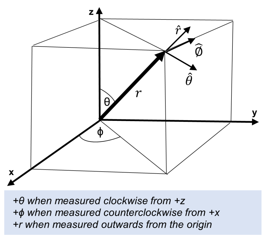
x=r\sin{\theta}\cos{\emptyset};
y=r\sin{\theta}\sin{\emptyset};
z=r\cos{\theta}
The unit vectors are:
\hat{r}=\frac{\vec{r}}{r}=\frac{x\hat{x}+y\hat{y}+z\hat{z}}{r}=\ \hat{x}\sin{\theta}\cos{\emptyset}+\hat{y}\sin{\theta}\sin{\emptyset}+\hat{z}\cos{\theta};
\hat{\theta}=\hat{\emptyset}\mathrm{\mathrm{\ x\ }}\hat{r}=\ \hat{x}\cos{\theta}\cos{\emptyset}+\hat{y}\cos{\theta}\sin{\emptyset}-\hat{z}\sin{\theta};
\hat{\emptyset}=\frac{\hat{z}\mathrm{\ x\ }\ \hat{r}}{\sin{\theta}}=-\hat{x}\sin{\emptyset}+\hat{y}\cos{\emptyset}
Since the unit vectors are not attached to the coordinate system axes, they are functions of time and can point in any direction. Therefore, they are not constant, and their time derivatives are not zero.
The time derivative of the unit vectors
\dot{\hat{r}}=\frac{\partial\hat{r}}{\partial r}\dot{r}+\frac{\partial\hat{r}}{\partial\theta}\dot{\theta}+\frac{\partial\hat{r}}{\partial\emptyset}\dot{\emptyset}=\ \dot{\theta\hat{\theta}}+\dot{\emptyset}\sin{\theta}\hat{\emptyset};
\dot{\hat{\theta}}=\frac{\partial\hat{\theta}}{\partial r}\dot{r}+\frac{\partial\hat{\theta}}{\partial\theta}\dot{\theta}+\frac{\partial\hat{\theta}}{\partial\emptyset}\dot{\emptyset}=\ -\dot{\theta\hat{r}}+\dot{\emptyset}\cos{\theta}\hat{\emptyset};
\dot{\hat{\emptyset}}=\frac{\partial\hat{\emptyset}}{\partial r}\dot{r}+\frac{\partial\hat{\emptyset}}{\partial\theta}\dot{\theta}+\frac{\partial\hat{\emptyset}}{\partial\emptyset}\dot{\emptyset}=-\left(\hat{r}\sin{\theta}+\hat{\theta}\cos{\theta}\right)\dot{\emptyset}
Velocity and Acceleration of a Point in Space (or a particle)
The position vector is given by: \vec{r}=r\hat{r} (1)
Assuming that r is not constant, the expression for the velocity of a point located at the tip of the position vector is:
\vec{v}=\dot{\vec{r}}=\dot{\hat{r}}r+\hat{r}\dot{r}
By replacing \dot{\hat{r}} we obtain the final expression for the velocity with the three components:
\vec{v}=\dot{r}\hat{r}+r\dot{\theta}\hat{\theta}+r\dot{\emptyset}\sin{\theta}\hat{\emptyset} (2)
Next, to obtain the expression for the acceleration, we differentiate the velocity with respect to time:
\vec{a}=\dot{r}\dot{\hat{r}}+\ddot{r}\hat{r}+r\dot{\theta}\dot{\hat{\theta}}+\dot{r}\dot{\theta}\hat{\theta}+r\ddot{\theta}\hat{\theta}+r\dot{\emptyset}\sin{\theta}\dot{\hat{\emptyset}}+\dot{r}\dot{\emptyset}\sin{\theta}\hat{\emptyset}+r\ddot{\emptyset}\sin{\theta}\hat{\emptyset}+r\dot{\emptyset}\dot{\theta}\cos{\theta}\hat{\emptyset}
By simplifying and ordering terms, we obtain the final expression for the acceleration:
\vec{a}=\left(\ddot{r}-r{\dot{\theta}}^2-r{\dot{\emptyset}}^2{sin}^2\theta\right)\hat{r}+\left(r\ddot{\theta}+2\dot{r}\dot{\theta}-r{\dot{\emptyset}}^2\sin{\theta}\cos{\theta}\right)\hat{\theta}+\left(r\ddot{\emptyset}\sin{\theta}+2r\dot{\theta}\dot{\emptyset}\cos{\theta}+2\dot{r}\dot{\emptyset}\sin{\theta}\right)\hat{\emptyset} (3)
Equation (3) shows the nine components of the acceleration, three for each direction. In general terms, we have:
\vec{a}=a_r\hat{r}+a_\theta\hat{\theta}+a_\emptyset\hat{\emptyset} (4)
Components of a Resultant Force in Space
Let’s suppose a body of ANY shape whose center of mass m is at the tip of the vector \vec{r}, as shown in the figure below. Let’s also assume that several forces are acting on the body and that the sum of all of them is the resultant force \vec{F} which points in a certain direction in space.
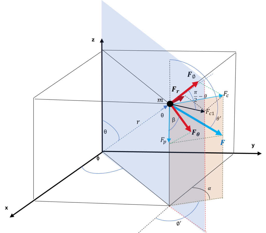
To find the components of this force in spherical coordinates, we have first to find its vertical and horizontal components ({\vec{F}}_c and {\vec{F}}_p), and then find the projections of them on the three spatial directions (\hat{r},\ \hat{\theta},\ \hat{\emptyset} ).
{\vec{F}}_c=F\cos{(\theta^\prime-\frac{\pi}{2})} (5)
{\vec{F}}_p=F\sin{(\theta^\prime-\frac{\pi}{2})} (6)
The Polar Component
This is the component of the force in the \hat{\theta} direction.
{\vec{F}}_\theta=F_p\cos{(\beta)}=F_p\cos{\left(\frac{\pi}{2}-\theta\right)=F_p\sin{\theta}}
By replacing F_p (Eq. 6):
{\vec{F}}_\theta=F\sin{\left(\theta^\prime-\frac{\pi}{2}\right)}{\sin{\theta}}
Applying trigonometric identities and simplifying, we get:
{\vec{F}}_\theta=F\cos{\theta^\prime}{\sin{\theta}}\ \ =\ \ \ \frac{F}{2}\left[\sin{\left(\theta^\prime+\theta\right)}+\sin{\left(\theta-\theta^\prime\right)}\right]\ \ =\ \ \ \frac{F}{2}\left[\sin{\left(\theta^\prime+\theta\right)}-\sin{\left(\theta^\prime-\theta\right)}\right]
We define the sum and difference of polar angles as:
| \theta_s=\left(\theta^\prime+\theta\right) | and | \theta_d=\left(\theta^\prime-\theta\right) |
The final expression of the polar force component is:
{\vec{F}}_\theta=\frac{F}{2}\left(\sin{\theta_s}-\sin{\theta_d}\right) (7)
The Azimuthal Component
This is the component of the force in the \ \hat{\emptyset} direction.
{\vec{F}}_\emptyset=F_c\cos{(\alpha)}=F_c\cos{\left(\pi-\emptyset^\prime\right)}
By replacing F_c (Eq. 1):
{\vec{F}}_\emptyset=F\cos{\left(\theta^\prime-\frac{\pi}{2}\right)}\cos{\left(\pi-\emptyset^\prime\right)}
Applying trigonometric identities, we get:
{\vec{F}}_\emptyset=-F\sin{\theta^\prime}\cos{\emptyset^\prime}\ =\ -\frac{F}{2}\left[\sin{\left(\theta^\prime+\emptyset^\prime\right)}+\sin{\left(\theta^\prime-\emptyset^\prime\right)}\right]
The final expression of the azimuthal force component is:
{\vec{F}}_\emptyset=-\frac{F}{2}\left[\sin{\left(\theta^\prime+\emptyset^\prime\right)}+\sin{\left(\theta^\prime-\emptyset^\prime\right)}\right] (8)
The Radial Component
This is the component of the force in the \ \hat{r} direction.
{\vec{F}}r=F_{c1}\cos{\left(\frac{\pi}{2}-\theta\right)} (9)
| {\vec{F}}_{c1}=F_c\cos{\left(\emptyset^\prime-\emptyset\right)} ; | {\vec{F}}_c=F\cos{\left(\theta^\prime-\frac{\pi}{2}\right)} |
By replacing {\vec{F}}_{c1} and {\vec{F}}_c in Eq. (9), we obtain:
{\vec{F}}_r=F\cos{\left(\theta^\prime-\frac{\pi}{2}\right)\cos{\left(\emptyset^\prime-\emptyset\right)}}\cos{\left(\frac{\pi}{2}-\theta\right)}
We define the difference of azimuthal angles as:
\emptyset_d=\left(\emptyset^\prime-\emptyset\right)
Applying trigonometric identities, we get:
{\vec{F}}_r=F\sin{\theta^\prime}\sin{\theta}\cos{\emptyset_d}\ =\ \ \frac{F}{2}\left[\cos{\left(\theta^\prime-\theta\right)}-\cos{\left(\theta^\prime+\theta\right)}\right]\cos{\emptyset_d}
The final expression of the radial force component is:
{\vec{F}}_r=\frac{F}{2}\left(\cos{\theta_d}-\cos{\theta_s}\right)\cos{\emptyset_d} (10)
The Resultant Force
The resultant force is given by sum of expressions (7), (8) and (10):
\vec{F}=F_r\hat{r}+F_\theta\hat{\theta}+F_\emptyset\hat{\emptyset} (11)
\vec{F}=\frac{F}{2}\left(\cos{\theta_d}-\cos{\theta_s}\right)\cos{\emptyset_d}\hat{r}+\frac{F}{2}\left(\sin{\theta_s}-\sin{\theta_d}\right)\hat{\theta}-\frac{F}{2}\left[\sin{\left(\theta^\prime+\emptyset^\prime\right)}+\sin{\left(\theta^\prime-\emptyset^\prime\right)}\right]\hat{\emptyset} (12)
| According to the second law of Newton, we have: | \vec{F}=m\vec{a} |
From Eq. (4) and Eq. (11), we can write:
F_r\hat{r}+F_\theta\hat{\theta}+F_\emptyset\hat{\emptyset}=m\left(a_r\hat{r}+a_\theta\hat{\theta}+a_\emptyset\hat{\emptyset}\right)
Which means:
| F_r=ma_r | F_\theta=ma_\theta | F_\emptyset=ma_\emptyset |
The Spatial Motion Caused by the Resultant Force – System of Three Differential Equations
By replacing the components from Eq. (3) and (12):
\frac{F}{2}\left(\cos{\theta_d}-\cos{\theta_s}\right)\cos{\emptyset_d}=m\left(\ddot{r}-r{\dot{\theta}}^2-r{\dot{\emptyset}}^2\sin^2\theta\right) (13)
\frac{F}{2}\left(\sin{\theta_s}-\sin{\theta_d}\right)=m\left(r\ddot{\theta}+2\dot{r}\dot{\theta}-r{\dot{\emptyset}}^2\sin{\theta}\cos{\theta}\right) (14)
-\frac{F}{2}\left[\sin{\left(\theta^\prime+\emptyset^\prime\right)}+\sin{\left(\theta^\prime-\emptyset^\prime\right)}\right]=m\left(r\ddot{\emptyset}\sin{\theta}+2r\dot{\theta}\dot{\emptyset}\cos{\theta}+2\dot{r}\dot{\emptyset}\sin{\theta}\right) (15)
These equations describe the radial motion (13), the polar motion (14), and the azimuthal motion (15).
This is a system of three differential equations that describe the motion in space resulting from the force \vec{F} applied on mass m.
Bibliography
1. A. K. T. Assis, “Relational Mechanics and Implementation of Mach’s Principle with Weber’s Gravitational Force” (Apeiron, Montreal, 2014). http://www.ifi.unicamp.br/~assis/Relational-Mechanics-Mach-Weber.pdf
2. Charles W. Lucas, Jr. “The Electrodynamic Origin of the Force of Gravity”, Part 1 (2008), Part 2 (2009), Part 3 (2009).
3. M. Tajmar and A. K. T. Assis, “Gravitational Induction with Weber’s Force”, Canadian Journal of Physics, Vol. 93, pp. 1571-1573 (2015). https://cdnsciencepub.com/doi/abs/10.1139/cjp-2015-0285
https://www.researchgate.net/publication/281539528_Gravitational_Induction_with_Weber%27s_Force
4. Charles W. Lucas, Jr., “The Universal Electrodynamic Force” (2011), PROCEEDINGS of the NPA.
5. A. K. T. Assis, “Gravitation as a Fourth Order Electromagnetic Effect”, Advanced Electromagnetism: Foundations, Theory and Applications, T. W. Barrett and D. M. Grimes (eds.), (World Scientific, Singapore, 1995). https://www.ifi.unicamp.br/~assis/gravitation-4th-order-p314-331(1995).pdf
6. Andre Koch Torres Assis, “Compliance of a Weber’s force law for gravitation with Mach’s principle” (1993). https://www.researchgate.net/publication/314995028_Compliance_of_a_Weber’s_force_law_for_gravitation_with_Mach’s_principle
7. A. K. T. ASS1S, “Deriving gravitation from electromagnetism”, Can. J. Phys. 70, 330 – 340 (1992). https://cdnsciencepub.com/doi/abs/10.1139/p92-054
http://www.ifi.unicamp.br/~assis/Can-J-Phys-V70-p330-340%281992%29.pdf