Raul Fattore
March 20, 2022
Table of Contents
Abstract
After some research on the web, I was not able to find any studies that answered questions like:
- Why do secondary masses orbit in the equatorial plane of the central mass?
- Why do many galaxies have spiral shapes?
- What is the real orbit of a secondary mass around the central mass? Even when Keppler laws are right, they only give geometrical relations. It can’t be serious to continue with the use of these laws nowadays.
- How can we better predict motion trajectories when some velocity components and/or mass change?
- Why study the Coriolis force or the Euler force separately, as isolated motions? They appear naturally in the general equations of motion and should not be considered isolated forces. They are just components of the main force.
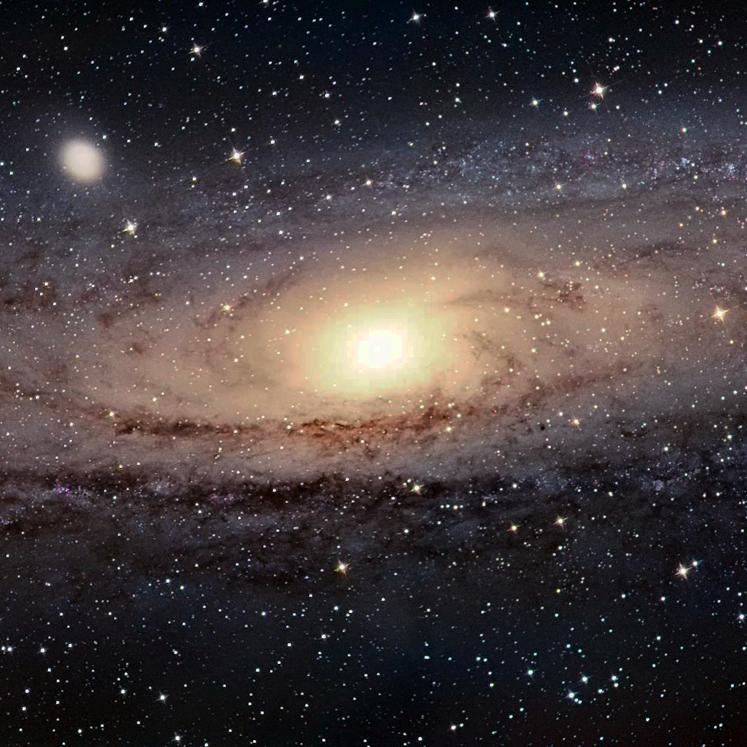
When we look at planets with their moons, our solar system, or distant galaxies, we see, in general, that the secondary masses orbit around the central mass mostly at its equatorial plane. If the present analysis is correct, then it gives the answer by demonstrating why this happens. It also demonstrates the spiral nature of the motion as well as the real orbit trajectories under diverse conditions. Moreover, it shows the motion modulation given by precession and/or nutation.
Introduction
The aim of this analysis is to provide a more efficient way to calculate and predict orbits and trajectories, not only for celestial bodies, but also for artificial satellites we send outside our atmosphere, and for ballistic. The equations presented here might also help improve weather forecasts and perhaps predict atmospheric behavior more precisely.
Nowadays, we know that gravity is an electromagnetic (EM) wave of atomic origin caused by a kind of dipole oscillation inside the atom [1]. This EM wave is always present in the universe as long as atoms exist and travels at the speed of light. When the originating mass of the EM gravity wave explodes or collapses, then a high amplitude EM gravity pulse is produced, which modulates the tail or final part of the regular wave. This pulse is the last message that we get from that mass.
We also know that the gravity field produced by a spinning central mass induces a motion on a secondary mass [2]. This induced motion has similar characteristics to that of the central mass.
I don’t have the knowledge to express gravity as a wave. Therefore, the present analysis is made based on the law of gravity according to Newton (instant action-at-a-distance). Just a pure mechanical study of the related free motion of two centers of mass in space, by considering all nine components of gravity acceleration. Even though gravity in this study is not considered as a wave (where time delay appears), the results are astonishing. However, the low velocities (compared with the speed of light) involved in the interaction of the free motion of two masses, make this study very suitable, except when the masses suddenly change, explode or collapse.
When I started the study, I did only analyze the motion in a single polar plane, without considering 3D spatial coordinates. I soon realized that this was a poor approach, not matching the real world. Then I switched to a spherical coordinate system to analyze the free motion between two centers of mass under the effects of gravity.
Motion in spherical coordinates
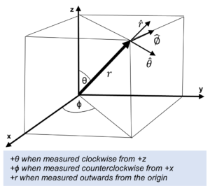
x=r\sin{\theta}\cos{\emptyset};
y=r\sin{\theta}\sin{\emptyset};
z=r\cos{\theta};
The unit vectors are:
\hat{r}=\frac{\vec{r}}{r}=\frac{x\hat{x}+y\hat{y}+z\hat{z}}{r}=\ \hat{x}\sin{\theta}\cos{\emptyset}+\hat{y}\sin{\theta}\sin{\emptyset}+\hat{z}\cos{\theta};
\hat{\theta}=\hat{\emptyset}\mathrm{\mathrm{\ x\ }}\hat{r}=\ \hat{x}\cos{\theta}\cos{\emptyset}+\hat{y}\cos{\theta}\sin{\emptyset}-\hat{z}\sin{\theta};
\hat{\emptyset}=\frac{\hat{z}\mathrm{\ x\ }\ \hat{r}}{\sin{\theta}}=-\hat{x}\sin{\emptyset}+\hat{y}\cos{\emptyset}
Since the unit vectors are not attached to the coordinate system axes, they are functions of time and can point in any direction. Therefore, they are not constant, and their time derivatives are not zero.
The time derivative of the unit vectors
\dot{\hat{r}}=\frac{\partial\hat{r}}{\partial r}\dot{r}+\frac{\partial\hat{r}}{\partial\theta}\dot{\theta}+\frac{\partial\hat{r}}{\partial\emptyset}\dot{\emptyset}=\ \dot{\theta\hat{\theta}}+\dot{\emptyset}\sin{\theta}\hat{\emptyset};
\dot{\hat{\theta}}=\frac{\partial\hat{\theta}}{\partial r}\dot{r}+\frac{\partial\hat{\theta}}{\partial\theta}\dot{\theta}+\frac{\partial\hat{\theta}}{\partial\emptyset}\dot{\emptyset}=\ -\dot{\theta\hat{r}}+\dot{\emptyset}\cos{\theta}\hat{\emptyset};
\dot{\hat{\emptyset}}=\frac{\partial\hat{\emptyset}}{\partial r}\dot{r}+\frac{\partial\hat{\emptyset}}{\partial\theta}\dot{\theta}+\frac{\partial\hat{\emptyset}}{\partial\emptyset}\dot{\emptyset}=-\left(\hat{r}\sin{\theta}+\hat{\theta}\cos{\theta}\right)\dot{\emptyset}
Velocity and Acceleration of a Point in Space (or a particle)
The position vector is given by: \vec{r}=r\hat{r} (1)
Assuming that r is not constant, the expression for the velocity of a point located at the tip of the position vector is:
\vec{v}=\dot{\vec{r}}=\dot{\hat{r}}r+\hat{r}\dot{r}
By replacing \dot{\hat{r}} we obtain the final expression for the velocity with the three components:
\vec{v}=\dot{r}\hat{r}+r\dot{\theta}\hat{\theta}+r\dot{\emptyset}\sin{\theta}\hat{\emptyset} (2)
Next, to obtain the expression for the acceleration, we differentiate the velocity with respect to time:
\vec{a}=\dot{r}\dot{\hat{r}}+\ddot{r}\hat{r}+r\dot{\theta}\dot{\hat{\theta}}+\dot{r}\dot{\theta}\hat{\theta}+r\ddot{\theta}\hat{\theta}+r\dot{\emptyset}\sin{\theta}\dot{\hat{\emptyset}}+\dot{r}\dot{\emptyset}\sin{\theta}\hat{\emptyset}+r\ddot{\emptyset}\sin{\theta}\hat{\emptyset}+r\dot{\emptyset}\dot{\theta}\cos{\theta}\hat{\emptyset}
By simplifying and ordering terms, we obtain the final expression for the acceleration:
\vec{a}=\left(\ddot{r}-r{\dot{\theta}}^2-r{\dot{\emptyset}}^2{sin}^2\theta\right)\hat{r}+\left(r\ddot{\theta}+2\dot{r}\dot{\theta}-r{\dot{\emptyset}}^2\sin{\theta}\cos{\theta}\right)\hat{\theta}+\left(r\ddot{\emptyset}\sin{\theta}+2r\dot{\theta}\dot{\emptyset}\cos{\theta}+2\dot{r}\dot{\emptyset}\sin{\theta}\right)\hat{\emptyset} (3)
Equation (3) shows the nine components of the acceleration, three for each direction. In general terms, we have:
\vec{a}=a_r\hat{r}+a_\theta\hat{\theta}+a_\emptyset\hat{\emptyset} (4)
Gravity as the Cause of the Acceleration
To analyze the free motion due to the gravity of a secondary mass with respect to a central mass, we must find the components of the gravitational acceleration in all three directions: \hat{r}, \hat{\theta}, and \hat{\emptyset}.
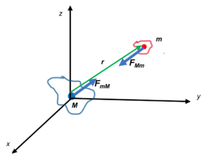
Let’s suppose a mass M of any shape, whose center of mass is at the origin of the coordinate system, and a mass m of any shape, whose center of mass is at a distance r from M. The attraction forces on them due to gravity are:
F_{mM}=-F_{Mm}=G\frac{m\ast M}{r^2}\hat{r}
Where G=6.67408\ast{10}^{-11}\ \frac{Nm^2}{Kg^2} is the universal gravitational constant.
Both centers of masses M and m may represent single bodies or distribution of several bodies.
The acceleration produced by M on m is given by: a_{Mm}=-G\frac{M}{r^2}\hat{r}, and the acceleration produced by m on M is given by: a_{mM}=G\frac{m}{r^2}\hat{r}.
We have two equal and opposite forces, but the accelerations are not equal. Working with two forces or two accelerations make things more complicated, and it is not helpful to analyze the interaction between the masses. How to find only one equation that describes the gravitational motion between the two bodies?
Gravity Interaction Between Two Masses Expressed With One Equation
We can make use of the second law of Newton, and express the force of gravity as:
F=m\vec{a}=m\frac{d^2r}{dt^2}\hat{r}=-G\frac{m\ast M}{r^2}\hat{r}
For mass M and m we can write:
M\frac{d^2r}{dt^2}\hat{r}=-G\frac{m\ast M}{r^2}\hat{r}
=>
\frac{d^2r}{dt^2}\hat{r}=-G\frac{m}{r^2}\hat{r} (5)
m\frac{d^2r}{dt^2}\left(-\hat{r}\right)=-G\frac{m\ast M}{r^2}\left(-\hat{r}\right)
=>
\frac{d^2r}{dt^2}\hat{r}=-G\frac{M}{r^2}\hat{r} (6)
Equation (5) is the acceleration produced by mass m, and Eq. (6) is the acceleration produced by mass M. By adding equations (5) and (6), we obtain:
2\frac{d^2r}{dt^2}\hat{r}=-G\frac{\left(M+m\right)}{r^2}\hat{r}
=>
\frac{d^2r}{{dt}^2}=-G\frac{\left(M+m\right)}{2}\frac{\hat{r}}{r^2}=a_{Gr}\hat{r} (7)
Equation (7) gives the interaction or relative motion between the two masses. It’s an average acceleration expressed by the average of the masses so that the relative acceleration produced by any one of the masses on the other has now the same value, which can be written as:
a_{avg}=-G\frac{m_{avg}}{r^2}\hat{r}
This way we can reduce our system to only one acceleration expression which accounts for the interaction of both masses.
For a big difference in masses (M>>m), as the mass of the Sun compared with the mass of the Earth (the mass of the Sun is 333,000 times greater), then the acceleration is mainly given by the bigger mass (Sun):
\frac{d^2r}{dt^2}=-G\frac{M}{2}\frac{\hat{r}}{r^2}
Components of the Gravity Acceleration in Spherical Coordinates
Equation (7) gives the acceleration of gravity in just one direction (\hat{r}). The general expression of the acceleration of gravity in spherical coordinates is:
{\vec{a}_G}=a_{Gr}\hat{r}+a_{G\theta}\hat{\theta}+a_{G\emptyset}\hat{\emptyset} (9)
Let’s find the remaining components of {\vec{a}}_G.
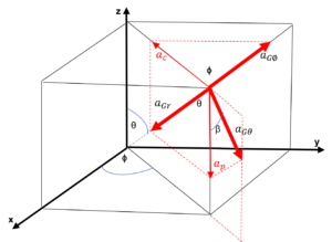
The centripetal acceleration a_c is the horizontal component of a_{Gr} parallel to the x-y plane and points to the z-axis, which will be rotating in a counterclockwise direction.
a_c=a_{Gr}\sin{\theta}
The projection of a_c in the direction of \hat{\emptyset} is the component a_{G\emptyset}:
a_{G\emptyset}=a_c\cos{\emptyset}
By replacing a_c we obtain the final expression for a_{G\emptyset}:
a_{G\emptyset}=a_{Gr}\sin{\theta}\cos{\emptyset} (10)
By replacing a_{Gr} from Eq. (7) in (10), we obtain the gravitational acceleration in the \hat{\emptyset} direction:
a_{G\emptyset}=-G\frac{\left(M+m\right)}{2{\ r}^2}\sin{\theta}\cos{\emptyset} (11)
The polar acceleration a_p is the vertical component of a_{Gr} parallel to the z-axis and points downwards when the vector \vec{r} is above the x-y plane or points upwards when the vector \vec{r} is below the x-y plane. This component is responsible for the pendulum-like motion of the center of mass m around the equatorial plane of the central mass M.
a_p=a_{Gr}\cos{\theta}
The projection of a_p in the direction of \hat{\theta} is the component a_{G\theta}:
a_{G\theta}=a_p\cos{\beta}
with \beta=\frac{\pi}{2}-\theta
=>
a_{G\theta}=a_p\cos{\left(\frac{\pi}{2}-\theta\right)}=a_p\sin{\theta}
By replacing a_p we obtain the final expression for a_{G\theta}:
a_{G\theta}=a_{Gr}\cos{\theta}\sin{\theta}
=>
a_{G\theta}=a_{Gr}\frac{\sin{\left(2\theta\right)}}{2} (12)
By replacing a_{Gr} from Eq. (7) in (12), we obtain the gravitational acceleration in the \hat{\theta} direction:
a_{G\theta}=-G\frac{\left(M+m\right)}{4\ r^2}\sin{\left(2\theta\right)} (13)
Inserting the components of the gravitational acceleration in Eq. (9), we get:
{\vec{a}}_G=-G\frac{\left(M+m\right)}{2{\ r}^2}\hat{r}-G\frac{\left(M+m\right)}{4\ r^2}\sin{\left(2\theta\right)}\hat{\theta}-G\frac{\left(M+m\right)}{2{\ r}^2}\sin{\theta}\cos{\emptyset}\hat{\emptyset} (14)
Relating The Motion With Its Cause
Now we can equate the equation of motion (4) with its cause (9):
\vec{a}={\vec{a}}_G
=>
a_r\hat{r}+a_\theta\hat{\theta}+a_\emptyset\hat{\emptyset}\ =\ a_{Gr}\hat{r}+a_{G\theta}\hat{\theta}+a_{G\emptyset}\hat{\emptyset}
We obtain a system of three differential equations that describe the full motion of the center of mass m relative to M:
a_r=\ a_{Gr}
a_\theta=\ a_{G\theta}
a_\emptyset=a_{G\emptyset}
Replacing all components:
\ddot{r}-r{\dot{\theta}}^2-r{\dot{\emptyset}}^2{sin}^2\theta=-G\frac{\left(M+m\right)}{2{\ r}^2} (15)
r\ddot{\theta}+2\dot{r}\dot{\theta}-r{\dot{\emptyset}}^2\sin{\theta}\cos{\theta}=-G\frac{\left(M+m\right)}{4\ r^2}\sin{\left(2\theta\right)} (16)
r\ddot{\emptyset}\sin{\theta}+2r\dot{\theta}\dot{\emptyset}\cos{\theta}+2\dot{r}\dot{\emptyset}\sin{\theta}=-G\frac{\left(M+m\right)}{2{\ r}^2}\sin{\theta}\cos{\emptyset} (17)
These equations describe the radial motion (15), the polar motion (16), and the azimuthal motion (17).
Radial Motion Differential Equation
We can write Eq. (15) as:
{\ddot{r}}{(t)}-r{\left(t\right)}{\dot{\theta}}{\left(t\right)}^2-r{\left(t\right)}{\dot{\emptyset}}{\left(t\right)}^2\sin^2\left(\theta{\left(t\right)}\right)+G\frac{\left(M+m\right)}{2{\ r}^2}=0
{\ddot{r}}{(t)}-\left[{\dot{\emptyset}}{\left(t\right)}^2{sin}^2\left(\theta_{\left(t\right)}\right)+{\dot{\theta}}{\left(t\right)}^2\right]\ r{\left(t\right)}+G\frac{\left(M+m\right)}{2r_{(t)}^2}=0 (18)
Polar Motion Differential Equation
We can write Eq. (16) as:
r_{\left(t\right)}{\ddot{\theta}}{(t)}+2{\dot{r}}{(t)}{\dot{\theta}}{\left(t\right)}-r{\left(t\right)}{\dot{\emptyset}}{\left(t\right)}^2\sin{\theta{(t)}}\cos{\theta_{(t)}}+G\frac{\left(M+m\right)}{4\ r_{(t)}^2}\sin{\left(2\theta_{(t)}\right)}=0;
{\ddot{\theta}}{(t)}+\frac{2{\dot{r}}{(t)}{\dot{\theta}}{\left(t\right)}}{r{\left(t\right)}}-{\dot{\emptyset}}{\left(t\right)}^2\frac{\sin{\left(2\theta{(t)}\right)}}{2}+G\frac{\left(M+m\right)}{4\ r_{(t)}^3}\sin{\left(2\theta_{(t)}\right)}=0;
{\ddot{\theta}}{(t)}+\frac{2{\dot{r}}{(t)}{\dot{\theta}}{\left(t\right)}}{r{\left(t\right)}}+\left[G\frac{\left(M+m\right)}{4\ r_{(t)}^3}-\frac{{\dot{\emptyset}}{\left(t\right)}^2}{2}\right]\sin{\left(2\theta{(t)}\right)}=0 (19)
Azimuthal Motion Differential Equation
We can write Eq. (17) as:
r_{(t)}{\ddot{\emptyset}}{(t)}\sin{\theta{(t)}}+2r_{(t)}{\dot{\theta}}{(t)}{\dot{\emptyset}}{(t)}\cos{\theta_{(t)}}+2{\dot{r}}{(t)}{\dot{\emptyset}}{(t)}\sin{\theta_{(t)}}+G\frac{\left(M+m\right)}{2{\ r}^2}\sin{\theta_{(t)}}\cos{\emptyset_{(t)}}=0;
{\ddot{\emptyset}}{(t)}+\frac{2r{(t)}{\dot{\theta}}{(t)}{\dot{\emptyset}}{(t)}\cos{\theta_{(t)}}}{r_{(t)}\sin{\theta_{(t)}}}+\frac{2{\dot{r}}{(t)}{\dot{\emptyset}}{(t)}\sin{\theta_{(t)}}}{r_{(t)}\sin{\theta_{(t)}}}+G\frac{\left(M+m\right)}{2r_{(t)}^2}\frac{\sin{\theta_{(t)}}\cos{\emptyset_{(t)}}}{r_{(t)}\sin{\theta_{(t)}}}=0;
{\ddot{\emptyset}}{(t)}+\frac{2{\dot{\theta}}{(t)}{\dot{\emptyset}}{(t)}\cos{\theta{(t)}}}{\sin{\theta_{(t)}}}+\frac{2{\dot{r}}{(t)}{\dot{\emptyset}}{(t)}}{r_{(t)}}+G\frac{\left(M+m\right)}{2r_{(t)}^3}\cos{\emptyset_{(t)}}=0;
{\ddot{\emptyset}}{(t)}+2\left[\frac{{\dot{\theta}}{(t)}}{\tan{\theta_{(t)}}}+\frac{{\dot{r}}{(t)}}{r{(t)}}\right]{\dot{\emptyset}}{(t)}+G\frac{\left(M+m\right)}{2r_{(t)}^3}\cos{\emptyset_{(t)}}=0 (20)
The System Of Differential Equations Of The Free Motion of Celestial Bodies Around a Central Mass
Now we have a system of three differential equations that describe the free motion in space resulting from the interaction of two masses.
Obs.: this is a system with three unknowns and must obviously be solved as such. Attempts to solve any equation as an isolated one, by just giving values to two unknown variables, is nonsense.
The angular velocity of translation of the center of mass m is {\dot{\emptyset}}_{(t)}=\Omega. We’ll assume that m doesn’t spin, but only revolves around M. We’ll also assume that the center of mass M at the origin of the coordinate system is spinning at an angular velocity \Omega_\phi, which means that our frame of reference is rotating at that speed as shown in the figure:
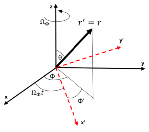
In the primed reference frame, we have:
| t^\prime=t | r^\prime=r | \theta^\prime=\theta | and | \phi^\prime=\phi-\Omega_\phi t |
Since the only difference is the relative angle, by differentiating we get the new relative angular velocity:
{\dot{\phi}}^\prime=\dot{\phi}-\Omega_\phi=\Omega-\Omega_\phi
The relative angular velocity could be zero, positive, or negative.
| {\dot{\phi}}^\prime=0 | could mean that the spin of M = translation velocity of m, or both angular velocities = 0. |
| {\dot{\phi}}^\prime<0 | is the case Sun-Earth or Earth-Moon. The spin of the Sun is faster than the translation’s angular speed of the Earth. The spin of the Earth is faster than the translation’s angular speed of the Moon. |
| {\dot{\phi}}^\prime>0 | another case for which I don’t have an example. |
In the system of differential equations (where only \dot{\phi} appears), we have just to change the initial conditions by replacing it with the proper relative angular velocity for each case. The variable \dot{\phi} represents the same as {\dot{\phi}}^\prime. The only difference is the value to be used in its initial condition.
If the mass M represents the mass of the Sun, we know that the period of one spin is ~ 25 days. Then its angular velocity is: \Omega_\phi=2.9\ {10}^{-6}[\frac{1}{s}]. The angular velocity of the Earth translation is:
\Omega=2\ {10}^{-7}[\frac{1}{s}]. Then the relative angular velocity between both masses is: \Omega-\Omega_\phi=-2.7\ {10}^{-6}[\frac{1}{s}]
Remarks About The Polar Motion
The differential equation of the polar motion (Eq. 22), has a term in brackets that can have three different values:
| \left[G\frac{\left(M+m\right)}{4\ r_{(t)}^3}-\frac{{\dot{\emptyset}}_{\left(t\right)}^2}{2}\right]=0 | => | G\frac{\left(M+m\right)}{2\ r_{(t)}^3}={\dot{\emptyset}}_{\left(t\right)}^2 | => | G\frac{\left(M+m\right)}{2\ r_{(t)}^2}={r_{(t)}\dot{\emptyset}}_{\left(t\right)}^2 |
| \left[G\frac{\left(M+m\right)}{4\ r_{(t)}^3}-\frac{{\dot{\emptyset}}_{\left(t\right)}^2}{2}\right]>0 | => | G\frac{\left(M+m\right)}{2\ r_{(t)}^3}>{\dot{\emptyset}}_{\left(t\right)}^2 | => | G\frac{\left(M+m\right)}{2\ r_{(t)}^2}>{r_{(t)}\dot{\emptyset}}_{\left(t\right)}^2 |
| \left[G\frac{\left(M+m\right)}{4\ r_{(t)}^3}-\frac{{\dot{\emptyset}}_{\left(t\right)}^2}{2}\right]<0 | => | G\frac{\left(M+m\right)}{2\ r_{(t)}^3}<{\dot{\emptyset}}_{\left(t\right)}^2 | => | G\frac{\left(M+m\right)}{2\ r_{(t)}^2}<{r_{(t)}\dot{\emptyset}}_{\left(t\right)}^2 |
We see that the cases above happen when the relative gravitational acceleration between the masses is equal to, greater than, or less than the centripetal acceleration of the center of mass m.
For a given relative angular velocity (translation of m-rotation of M), the equations above will give the distance:
| r_{(t)}=\sqrt[3]{G\frac{\left(M+m\right)}{2\ {\dot{\emptyset}}_{\left(t\right)}^2}} | r_{(t)}<\sqrt[3]{G\frac{\left(M+m\right)}{2\ {\dot{\emptyset}}_{\left(t\right)}^2}} | r_{(t)}>\sqrt[3]{G\frac{\left(M+m\right)}{2\ {\dot{\emptyset}}_{\left(t\right)}^2}} | (24) |
The first term of the acceleration in the brackets gives a curious result when we substitute the values of the mass of the Sun in M, the mass of the Earth in m, and the distance Sun-Earth in r.
G\frac{\left(M+m\right)}{4\ r_{(t)}^3}=\frac{6.67408\ {10}^{-11}\left(2{\ 10}^{30}+5.9\ {10}^{24}\right)}{4\ \left(150\ {10}^9\right)^3}=9.887555\ {10}^{-15}\ \ \left[\frac{1}{s^2}\right]
This angular acceleration is a small fraction of the gravitational acceleration on the Earth’s surface.
Solving The System of Three Differential Equations
Finding the solutions of the system of differential equations (21), (22), and (23) is not an easy task, and requires the use of some software for Mathematics and Physics applications. Numerical solutions were obtained by using a Runge-Kutta method, as well as several plots that describe the behavior of the free motion in space due to the gravitational interaction between two centers of masses under diverse initial conditions. The results are astonishing.
However, as some calculations might take days on a regular PC, in order to confirm some conclusions, a much more powerful computer is needed to evaluate the motion under certain conditions, and for very long times.
Nevertheless, in most cases, the calculations and the resolution of the graphics were satisfactory for the present analysis.
The system of Differential equations (21), (22), and (23), describe the relative free motion of ANY two centers of masses M and m under the action of gravity acceleration. The centers of masses can represent single bodies or a group of bodies of any shape.
To make calculations with real values, the masses of the Sun and Earth, as well as distances like Sun-Earth were used in the system of differential equations. It could also have been the interaction between Andromeda and the Milky Way, or a human artificial satellite and Earth, or whatever two (centers of) masses one may think about.
Therefore, in the present study, we have a central mass M which is much bigger than the secondary mass m, that is M >> m.
Results show that in most of the cases, the center of mass m reaches equilibrium around the equatorial plane of the central mass M, i.e., \theta\approx90^{\circ}.
There are only a few cases where m reaches equilibrium at \theta\approx0^{\circ} (+ z-axis), \theta\approx180^{\circ} (- z-axis), and other polar angular positions.
Results
First, general results were obtained with initial conditions for three different relative azimuthal angular velocities (\dot{\phi}), which give three different initial positions of the vector r_{(t)} as given by equations (24). Thus, we can check the behavior of the motion by giving the term in brackets of Eq. (22) three different values: zero, positive or negative. See Table 1.
Next, a similar analysis was performed, but exclusively for polar initial positions different of zero. See Table 2.
The final analysis shown in Table 3 was made to check the motion behavior at rather short and long distances between the two centers of masses.
Parameters and Common Initial Conditions
| G=6.67408\ast{10}^{-11}\ \frac{Nm^2}{{\rm Kg}^2} | (the universal gravitational constant) |
| M=2\ {10}^{30}\ Kg | (the mass of the Sun) |
| m=5.9\ {10}^{24}\ Kg | (the mass of the Earth) |
| {\dot{r}}_{(0)}=0\ [m/s] | (linear velocity of the center of mass m at t=0) |
| \emptyset_{(0)}=0\ [rad] | (azimuthal position of the center of mass m at t=0) |
| {\dot{\emptyset}}_{(t)}=\Omega | (is the relative angular velocity between the spin of the center of mass M and the translation of the center of mass m) |
Since there is a singularity for \theta=0, the “zero” initial condition of the polar angle was taken close to zero as \theta=\frac{\pi}{{10}^3}\ [rad].
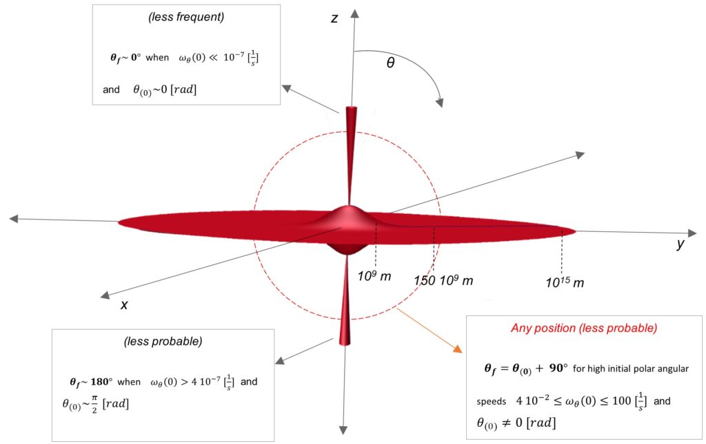
Scheme of Positions of Mass m in Function of the Distance to Mass M, according to results
An approximate scheme (not in scale) based on the results of Table 1, Table 2, and Table 3, which illustrates most of the positions that mass m can adopt with respect to the distance (r) to mass M located at the origin of coordinates.
Comments About The Results
Even when the results of the present study were obtained with a limited set of initial conditions, they are in close agreement with observations of the universe, and what mother nature shows us.
Recall that the polar component of the gravity acceleration on mass m points downwards in the upper hemisphere, and points upwards in the lower hemisphere.
Then, it is somewhat logical to expect a pendulum-like motion in the polar direction, that may “force” mass m to stay approximately in the equatorial plane, or x-y plane. The universe shows that this is the general case.
However, if the distance is short between the masses, then the secondary mass (m), depending on its initial angular position, may adopt any position around mass M. In this region \theta_f=\theta_{(0)}. The universe also shows that this is the general case.
According to what the universe shows us, one may classify some positions as “less frequent” and “less probable”. In these cases, the initial conditions that gave such results could also be “less frequent” and “less probable” to happen in the universe.
In general, the center of mass m can reach its equilibrium or stable final position, in two ways: by approaching the final position asymptotically, or by oscillating. When oscillations are present, they are mostly modulated in amplitude by a lower frequency motion, which I believe could be due to the precession of mass M. This lower frequency motion modulation is, in general, also of variable frequency. So, we have both: amplitude and frequency modulation of the motion.
There are also some unstable solutions of the motion (resonance), or because of some singularity, where amplitude increases steadily. There is no real equilibrium or stable final position in these cases.
Precession and Nutation – Not Always Present
Before the present study, I thought that Precession and Nutation were characteristic motions of any spinning body.
Surprisingly, some results show that the center of mass m not always reaches the equilibrium position with an oscillatory motion, but asymptotically. Precession and Nutation are absent in such cases.
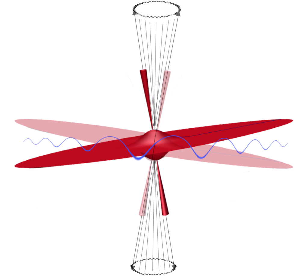
For simplicity, Precession and Nutation motions are not shown in the scheme of the positions of mass m, but they might be present in spinning bodies under certain conditions. In such cases, the center of mass m at equilibrium will follow those motions.
The z-axis will describe an oscillatory cone-like trajectory. In the x-y plane, the motion will be like a wobbling dish or coin on a table. Since gravitational acceleration is an EM wave [1], the motion will be subject to a delay in function of the distance between both centers of masses.
Conclusions
The present study demonstrates that in most cases, the secondary mass orbits in the equatorial plane of the main central mass.
It is also shown the real orbit trajectories and the spiral nature of the motion.
Additionally, it is also demonstrated that the motion modulation caused by precession and/or nutation is not always present. I don’t have access to high computation capacity clusters to validate some conclusions. The use of powerful computation machines is advisable for this study. However, the performed calculations and plots in this analysis are more than satisfactory to make conclusions.
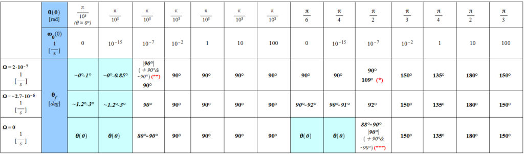
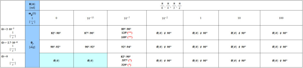
Table 1 – General Results
The calculations were made for three initial positions of the vector r(t):
| r_{(0)}=1.186071579\ {10}^{11}\ [m] | r_{(0)}=100\ {10}^9\ [m] | r_{(0)}=150\ {10}^9\ [m] | (distance Sun-Earth) |
(*): result for r=150\ast{10}^9[m] and \Omega=2\ast{10}^{-7}[\frac{1}{s}]
(**): result for r=1.186071579\ \ast\ {10}^{11}[m] and \Omega=2\ast{10}^{-7}[\frac{1}{s}]
(***): result for r=100\ast{10}^9[m] and \Omega=0[\frac{1}{s}]
Note:
1. Results are the same for the three initial position values of r_{(0)}, except for (*), (**), and (***).
2. In general, the final polar position is given by \theta_f=\theta_{(0)}+90^{\circ}, except for the colored table cells, where the final position is \theta_f=\theta_{(0)}, when the initial value of the polar angular velocity \omega_\theta(0) is very low or zero.
See the Plots of the Results Summarized in Table 1 for details of the motion of mass m around a central mass M according to the shown initial conditions.
Table 2 – Results only for initial polar positions θ(0) ≠ 0 of the center of mass m
The calculations were made for three initial positions of the vector r(t):
| r_{(0)}=1.186071579\ {10}^{11}\ [m] | r_{(0)}=100\ {10}^9\ [m] | r_{(0)}=150\ {10}^9\ [m] | (distance Sun-Earth) |
There is a “critical” \omega_\theta(0) for which the mass m reaches the equilibrium away from 90^{\circ}. This value is around {3*{10}^{-7}<\omega}_\theta(0)<4\ast{10}^{-7}[\frac{1}{s}]
(*): the plot cannot be done beyond a certain point because of a probable singularity. The angle increases steadily, and it is impossible to see an equilibrium or a final stable angle.
(**): results for r=150\ast{10}^9[m], \theta_{(0)}=\frac{\pi}{3} and \theta_{(0)}=\frac{\pi}{2} respectively
Note:
1. Results are quite the same for the four initial position values of \theta_{(0)} and the three initial position values of r_{(0)}, except for (*) and (**).
2. In general, for initial values of the polar angular velocity \omega_\theta(0)>4\ast{10}^{-7}[\frac{1}{s}], the final polar position is given by \theta_f=\theta_{(0)}+90^{\circ}. We also observe two cases on the colored table cells on the left, where the final position is \theta_f=\theta_{(0)} when the initial value of the polar angular velocity \omega_\theta(0) is very low or zero.
See the Plots of the Results Summarized in Table 2 for details of the motion of mass m around a central mass M according to the shown initial conditions.
Table 3 – Results for a short and long-distance (r) between the two centers of masses
The calculations were made for two initial positions of the vector r(t):
| {r1}_{(0)}={10}^9[m] | and | {r2}_{(0)}={10}^{15}[m] |
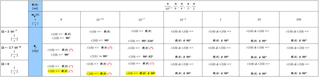
(“): there is some discontinuity for all the initial positions of the polar angle. In some cases, it was taken the average value of the angle. In other cases, it was considered the maximum value of the angle before the discontinuity, since the angle increases steadily.
(*): there is some discontinuity only at the initial position \theta_{(0)}=\frac{\pi}{{10}^3} of the polar angle. It was taken the maximum value of the angle before the discontinuity, since the angle increases steadily.
Note:
1. Results are the same for the five initial position values of \theta_{(0)} and the two initial position values of r(0), when \omega_\theta(0)>4\ast{10}^{-7}[\frac{1}{s}]. Results are also the same for \omega_\theta(0)<4\ast{10}^{-7}[\frac{1}{s}] and for r1(0), except for (“) and (*), where the final polar angle is given by \theta_f=\theta_{(0)} when the initial value of the polar angular velocity \omega_\theta(0) is very low or zero. However, for r2(0) we have three cases that differ of the rest, as shown in the highlighted values.
2. In general, for initial values of the polar angular velocity \omega_\theta(0)>4\ast{10}^{-7}[\frac{1}{s}], the final polar position is given by \theta_f=\theta_{(0)}+90^{\circ}.
See the Plots of the Results Summarized in Table 3 for details of the motion of mass m around a central mass M according to the shown initial conditions.
Bibliography
[1] A. K. T. Assis, “Gravitation as a Fourth Order Electromagnetic Effect”, Advanced Electromagnetism: Foundations, Theory and Applications, T. W. Barrett and D. M. Grimes (eds.), (World Scientific, Singapore, 1995). https://www.ifi.unicamp.br/~assis/gravitation-4th-order-p314-331(1995).pdf
[2] M. Tajmar and A. K. T. Assis, “Gravitational Induction with Weber’s Force”, Canadian Journal of Physics, Vol. 93, pp. 1571-1573 (2015). https://cdnsciencepub.com/doi/abs/10.1139/cjp-2015-0285
https://www.researchgate.net/publication/281539528_Gravitational_Induction_with_Weber%27s_Force
3. Charles W. Lucas, Jr. “The Electrodynamic Origin of the Force of Gravity”, Part 1 (2008), Part 2 (2009), Part 3 (2009).
4. A. K. T. Assis, “Relational Mechanics and Implementation of Mach’s Principle with Weber’s Gravitational Force” (Apeiron, Montreal, 2014). http://www.ifi.unicamp.br/~assis/Relational-Mechanics-Mach-Weber.pdf
5. Charles W. Lucas, Jr., “The Universal Electrodynamic Force” (2011), PROCEEDINGS of the NPA.
6. William D. Walker, “Superluminal Electromagnetic and Gravitational Fields
Generated in the Nearfield of Dipole Sources” (2006). https://arxiv.org/ftp/physics/papers/0603/0603240.pdf
7. V Pustovoit et al 2020 J. Phys.: Conf. Ser. 1557 012034, “High frequency gravitational waves generation by optical methods” (2020). https://iopscience.iop.org/article/10.1088/1742-6596/1557/1/012034/pdf
8. M. Tajmar, “Revolutionary Propulsion Research at TU Dresden” (2017). https://www.researchgate.net/publication/314238291_Revolutionary_Propulsion_Research_at_TU_Dresden
https://tu-dresden.de/ing/maschinenwesen/ilr/rfs/ressourcen/dateien/forschung/folder-2007-08-21-5231434330/ag_raumfahrtantriebe/SSI-Revolutionary-Propulsion-Research-at-TU-Dresden.pdf?lang=en
9. Andre Koch Torres Assis, “Compliance of a Weber’s force law for gravitation with Mach’s principle” (1993). https://www.researchgate.net/publication/314995028_Compliance_of_a_Weber’s_force_law_for_gravitation_with_Mach’s_principle
10. Robert M L Baker, Jr. and Bonnie Sue Baker, “Gravitational wave generator apparatus”, Physics Procedia 38 (2012) 288 – 297. https://www.researchgate.net/publication/276078203_Gravitational_Wave_Generator_Apparatus/fulltext/55dd373208ae591b309ac914/Gravitational-Wave-Generator-Apparatus.pdf
11. A. K. T. ASS1S, “Deriving gravitation from electromagnetism”, Can. J. Phys. 70, 330 – 340 (1992). https://cdnsciencepub.com/doi/abs/10.1139/p92-054
http://www.ifi.unicamp.br/~assis/Can-J-Phys-V70-p330-340%281992%29.pdf
12. S. Hacyan, “Gravitational radiation from a rotating magnetic dipole” (2017), Revista Mexicana de Fisica vol.63 no.5 México sep./oct. 2017. http://www.scielo.org.mx/scielo.php?script=sci_arttext&pid=S0035-001X2017000500466
Related articles:
Dynamic Deformation of Earth and Motion Effects Caused by Universe Gravitational Field