Intensity Of Electromagnetic Waves As a Function Of Frequency, Source Distance and Aperture Angle

Raul Fattore

March 23, 2022

Table of Contents

Abstract

Intensity of Electromagnetic Waves as a function of frequency is usually not treated by the scientific community.

The energy transport in Electromagnetic Waves (EMW) calculated by means of the Poynting vector formula, might not yield to correct results, because it only gives an average energy on a surface. There is no reference about the volumetric energy distribution at a distance from the source, nor to the frequency of the EMW.

How can the intensity of EMW be written in terms of frequency and distance to the source?
How to calculate the volumetric energy of EMW?
How does the intensity change with the aperture angle (solid angle of a cone in space) from the source?
How to relate intensity with frequency, area, and aperture angle in one equation?
How to obtain the wave equation of the interference caused by slit diffraction to compute the Intensity?

In this study, you’ll find the answers to the questions above and learn that the result obtained here agrees to the famous Planck equation ( $E=hf$ ). Moreover, a wave equation for the interference pattern produced by slit diffraction is obtained, but calculation of pattern intensities is left for you with the given formulas.

Introduction

We know that EMW transport energy in the form of alternating electric and magnetic fields, and even momentum, which is the cause of radiation pressure. Since pressure is force per unit area, the lesser the area, the greater the pressure.

The radiation per unit area of EMW is of extreme importance in physics, whether in generation or measurements of waves. You don’t need a laser to prove that. Just put a glass lens under the sun and a piece of paper at the lens focal plane and see what happens.

Most of the scientific publications and books treat energy measurement of EMW with the Poynting vector formula, that only contains the amplitude of the radiation. If you calculate two radiations of the same amplitude but different frequencies, the result obtained with the Poynting formula is the same. But this is not true, because the energy of the wave is directly proportional to the frequency.

Moreover, the energy is inversely proportional to the solid angle of a cone in space measured from the source, and this is valid for generated as well measured EMW.

Energy Transport in Electromagnetic Waves

The energy density (energy per unit volume) of the electric field is given by the following equation:

$u_E=\ \frac{1}{2}\varepsilon_0E_{(r,\ t)}^2$

On the other hand, the energy density of the magnetic field is given by:

$u_B=\ \frac{B_{(r,\ t)}^2}{2\mu_0}$

These equations show that in a region of empty space where $\vec{E}$ and $\vec{B}$ fields are present, the total energy density is given by:

$u=\ \frac{1}{2}\varepsilon_0E_{(r,\ t)}^2+\ \frac{B_{(r,\ t)}^2}{2\mu_0}$ (1)

Since $E$ and $B$ are related by $E_{(r,\ t)}=cB_{(r,\ t)}$ , then by replacing this in (1) we can write the energy density in function of the magnetic field:

$u=\ \frac{1}{2}\varepsilon_0c^2B_{(r,\ t)}^2+\ \frac{B_{(r,\ t)}^2}{2\mu_0}\ \ =\ \ \frac{1}{2}\varepsilon_0\frac{1}{\mu_0\varepsilon_0}B_{(r,\ t)}^2+\ \frac{B_{(r,\ t)}^2}{2\mu_0}$

$u=\frac{B_{(r,\ t)}^2}{\mu_0}$ (2)

(energy density in $\left[\frac{J}{m^3}\right]$ )

If we want the energy density given by the electric field, then we replace $B_{(r,\ t)}=\frac{E_{(r,\ t)}}{c}$ in (1):

$u=\ \frac{1}{2}\varepsilon_0E_{(r,\ t)}^2+\ \frac{E_{(r,\ t)}^2}{2{c^2\mu}0}\ \ =\ \ \ \frac{1}{2}\varepsilon_0E{(r,\ t)}^2+\ \frac{E_{(r,\ t)}^2\mu_0\varepsilon_0}{2\mu_0}$

$u=\varepsilon_0E_{(r,\ t)}^2$ (3)

(energy density in $\left[\frac{J}{m^3}\right]$ )

This shows that in vacuum, the total energy density of the wave can be associated whether with the $\vec{E}$ field or the $\vec{B}$ field.

Intensity – The Poynting Vector

The rate of energy transport per unit area or power per unit area or Intensity in such a wave is described by a vector $\vec{S}$ , called the Poynting vector.

Consider a static plane, perpendicular to the x-axis that coincides with the wave front at a certain time. In a time $dt$ after this, the wave front moves a distance $dx=c\ dt$ ahead of the plane.

If we take an area A on this static plane, we see that the energy in the space ahead of this area pass through the area to the new location. The volume $dV$ of this region is the area A multiplied by the length $c\ dt$ , and the energy $dU$ in this space is the energy density $u$ multiplied by this volume:

$dU=u\ dV={(\varepsilon}_0E_{(r,\ t)}^2)(Ac\ dt)$

As this energy passes through the area A in time $dt$ , the energy flow per unit time per unit area, which we will call intensity or S is:

$S=\frac{1}{A}\frac{dU}{dt}=\varepsilon_0cE_{(r,\ t)}^2$

$\left[\frac{W}{m^2}\right]$

By replacing $c$ , we obtain:

$S=\frac{\varepsilon_0}{\sqrt{\varepsilon_0\mu_0}}E_{(r,\ t)}^2=\sqrt{\frac{\varepsilon_0}{\mu_0}}E_{(r,\ t)}^2=\frac{E_{(r,\ t)}B_{(r,\ t)}}{\mu_0}$

$S=\frac{E_{(r,\ t)}B_{(r,\ t)}}{\mu_0}$ (4)

(magnitude of the power per unit area or Intensity in vacuum)

The vector quantity that describes the magnitude and direction of the energy flow rate, is the Poynting vector:

$\vec{S}=\frac{1}{\mu_0}\vec{E}\times\vec{B}$ (5)

(Poynting vector in vacuum)

Where the magnitude of the Poynting vector is given by (4).

The total energy flow per unit time (power, P) out of any closed surface is the integral of over the surface:

$P=\oint{\vec{S}\ d\vec{A}}$

Let’s suppose that we have an Electromagnetic wave with the following characteristic:

$E_y\left(r,t\right)=E_{max}\cos{(kr-\omega t)}$

$B_z\left(r,t\right)=B_{max}\cos{(kr-\omega t)}$

Now let’s calculate the intensity of this sinusoidal wave by using the Poynting vector formula.

$\vec{S}(r,t)=\frac{1}{\mu_0}\vec{E}(r,t)\times\vec{B}(r,t)=\hat{j}E_{max}\cos{(kr-\omega t)}\times\hat{k}B_{max}\cos{(kr-\omega t)}$

The vector product of the unit vectors is $\hat{j}\times\hat{k}=\hat{i}$ and $\cos^2{(kx-\omega t)}$ is never negative, so $\vec{S}(r,t)$ in this case always points in the positive x-direction (the direction of wave propagation). The x-component of the Poynting vector is:

$\vec{S}(x,t)=\frac{E_{max}B_{max}}{\mu_0}\cos^2{(kx-\omega t)}$

The time average value of $\cos^2{(kx-\omega t)}$ is $\frac{1}{2}$ . So, the average value of the Poynting vector or Intensity over a full cycle is ${\vec{S}}{av}=\hat{i}{\ S}{av}$ , where:

${\ S}{av}=\frac{E{max}B_{max}}{2\mu_0}=I$ (6)

By using the relationships $E_{max}=c\ B_{max}$ and $\varepsilon_0\mu_0=\frac{1}{c^2}$ we can express the intensity in several equivalent forms:

$I=\frac{{E_{max}}^2}{2\mu_0c}$ (7)

$I=\frac{1}{2}\varepsilon_0c{E_{max}}^2$ (8)

In addition, we can write the Intensity in terms of $E_{rms}$ , the root-mean-square value of the electric field.

$E_{rms}=\frac{E_{max}}{\sqrt2}$

By replacing this in Eq. (7), we get the Intensity in function of the $E_{rms}$ .

$I=\frac{1}{\mu_0c}E_{rms}^2$ (9)

Equations (7), (8) and (9) give different expressions to calculate the Intensity of EMW in vacuum.

Volumetric Power and Intensity of Electromagnetic Waves

The energy density ( $\left[\frac{J}{m^3}\right]$ ) of a wave in vacuum is given by Eq. (2) or Eq. (3). By definition, the energy transfer rate is given by the Power. Since we are considering a volume in space, it would be perfectly normal to find the Volumetric Power. With this, the Intensity of EMW is redefined to account for the energy in that volume.

The Power Density or Volumetric Power $P_v$ is the rate at which the energy is transferred: $P=\frac{\partial u}{\partial t}$ , where $u=\varepsilon_0E_{(r,\ t)}^2$ is the energy density in $\left[\frac{J}{m^3}\right]$ . Then, the Intensity can be redefined as the volumetric energy flow per unit time per unit area:

$I=\frac{P_v}{A}\ \ =\ \ \frac{1}{A}\frac{\partial u}{\partial t}$

$\left[\frac{\frac{W}{m^3}}{m^2}\right]$ (10)

How Intensity Changes with Distance and Area

Unfortunately, almost all scientific publications and books do not give any mathematical approach about the behavior of EMW when frequency and distance are considered. The Poynting vector basically ignores these factors, and the intensities obtained by this method are incorrect, because they do not match with Mather Nature.

The Poynting vector in Eq. (4) to (9) only give the average energy on a surface, with no reference to distance from the source nor to the frequency of the wave.

I have obtained more useful formulas that show how the energy of EMW depend on the wave’s frequency, the attenuation with the distance from the source, as well as how the intensity depends on the aperture angle (solid angle of a cone in space) between the source and the region in space where calculations or measurements are performed.

Energy Spread in EMW

I assume a small source that emits EMW isotropically. The spherical wave fronts spreading from such an isotropic point source S at a particular instant are shown in cross-section in the figure.

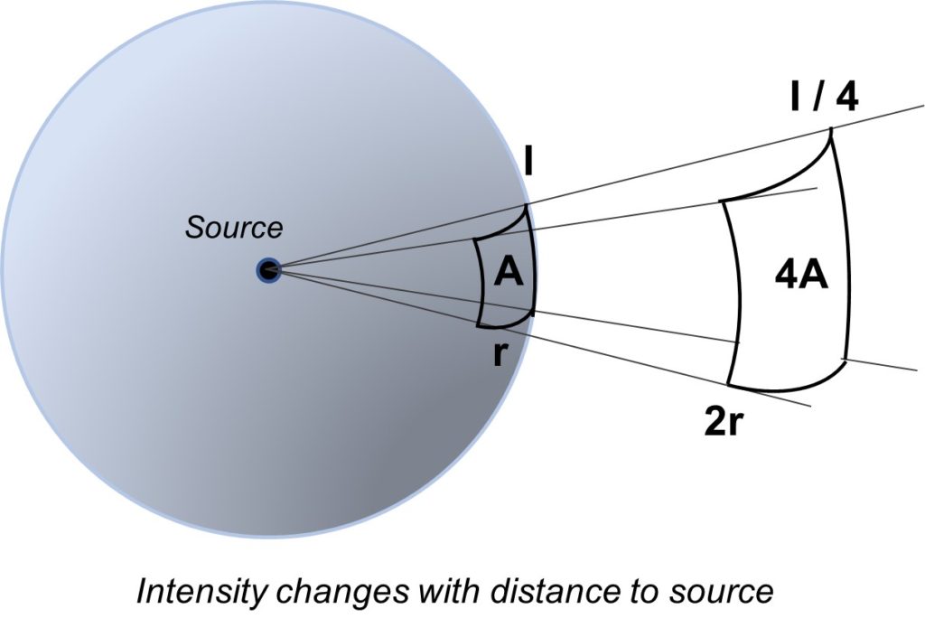
Let’s also assume that the energy of the waves is conserved as they spread from the source, and all the energy emitted must pass through the sphere.

Thus, the rate at which energy passes through the sphere as radiation must be equal to the rate at which the energy is emitted, that is, the source power Ps. The intensity I (power per unit area) measured at the sphere must then be, from Eq.(10):

$I=\frac{P_s}{{4\pi R}^2}$ (11)

Equation (11) tells us that the intensity of the electromagnetic radiation from an isotropic small source decreases with the square of the distance R from the source. Note that this is the intensity spread out all over the area of the sphere. It is only useful to demonstrate how the distance affect the intensity, and that’s all. Some unanswered questions are:

What happens in a small area of the sphere?
How does Intensity change with the aperture angle between the source and the observation region?
Does Intensity vary as frequency changes?

Calculation of a Cap Area of the Sphere

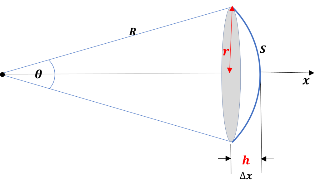
The cap area of a sphere is given by the following formula:

$A=\pi(h^2+r^2)$ (12)

If $R\gg r$ , we can make $\Delta_x$ very small, so that $h\ll r$ . Then, the cap area will be:

$A\approx\pi\ r^2$ (13)

That is, the area of the cap is practically the area of the circle of radius $r$ . The arc length is practically the same as the diameter, i.e.

$S\cong2r$

By definition, angle is the ratio of the arc to the radius: $\theta=\frac{S}{R}$

If we make $R\gg r$ , then the angle $\theta$ will be very small. For $\theta<0.2[rad]$ , which corresponds to $\theta\cong<10^{\circ}$ , and with an error $<1\%$ , we have:

$\tan{\left(\frac{\theta}{2}\right)\cong}\frac{\theta}{2}=\ \frac{r}{R}$

therefore

$r=\frac{\theta}{2}R$ (14)

Replacing (14) in (13), we get the following equation for the small cap area in function of the aperture angle and the distance from the origin:

$A=\frac{\pi}{4}\theta^2R^2$ (15)

Intensity Ratio Between Two Spherical Areas

Let’s imagine a small sphere tight surrounding the wave source, with an area $A_s$ and radius $r_s$ . Now consider another sphere at a distant point $x$ from the source, with area $A_x$ and radius $r_x$ .

The intensity at the source sphere will be:

$I_s=\frac{P_s}{A_s}$

And the intensity at the distance $x$ is:

$I_x=\frac{P_s}{A_x}$

The ratio of the intensity at the distance $x$ with respect to the source is:

$\frac{I_x}{I_s}=\frac{\frac{P_s}{A_x}}{\frac{P_s}{A_s}}=\frac{A_s}{A_x}$

then

$I_x=I_s\frac{A_s}{A_x}=\frac{4\pi{r_s}^2}{4\pi{r_x}^2}$

It follows that:

$I_x=I_s\left(\frac{r_s}{r_x}\right)^2$ (16)

Since $r_x>r_s$ , then $I_x<I_s$ , i.e., the intensity at the distance weakens by a factor $\frac{1}{r^2}$ .

Intensity Ratio Between a Small and Big Area Located at the Same Radius

Let’s imagine that we take a sphere of radius R and area $A_r$ at a big distance from the wave source. The intensity will be $I_r$ . Now, let’s take a very small area in the same sphere (a small sphere cap), so that its area is given by Equation (15).

The intensity for the whole area of the sphere is $I_r=\frac{P_s}{A_r}$ , and the intensity for the cap area is $I_{cap}=\frac{P_s}{A_{cap}}$ .

By taking the ratio of the intensities, it follows that:

$I_{cap}=I_r\frac{A_r}{A_{cap}}$

After replacing the area values, we obtain:

$I_{cap}=I_{r\ }\frac{4\piR^2}{\frac{\pi}{4}\theta^2R^2}$

Then, the intensity at the small cap area is given by:

$I_{cap}=I_r\frac{16}{\theta^2}$ (17)

Since the value of the angle is $\theta<0.2[rad]$ , then the intensity at the cap is, at least $I_{cap}=400\ I_r$ !

This remarkable result tells us that the smaller the angle, the bigger the intensity we can generate, measure, or detect. If we manage to concentrate and collimate the flux of measured or generated energy in a beam with a small aperture angle, then we may expect a huge gain in intensity.

The Magnifying Glass Effect and the Laser Power

The magnification factor in Equation (17) $F_\theta=\frac{16}{\theta^2}$ can be applied on emission and detection of EMW. Among other things, it explains the effect of a magnifying glass when burning a piece of paper on the sun by concentrating the sun energy in a small spot on the paper.

Another example is Laser. Laser light is collimated in a very small diameter beam of light, thus helping to obtain very high intensities.

In general, any type of emission and reception of EMW where the energy is confined in a small area, will take advantage of this fact. Some examples are systems using directional emission or detection with parabolic antennas, like radar, broadcasting, telephony, etc.

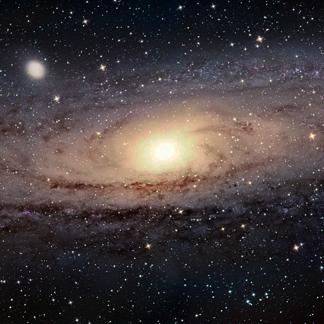
In astronomy, to detect extremely weak EMW coming from very distant stars or galaxies, we should need to capture as much energy as possible and focus the beam at a spot as small as possible, in order to get a minimum level of intensity capable of being observed and measured.

How Intensity Changes with Frequency, Distance, and Area

Recall that the volumetric power per unit area (Intensity) is the flow of energy per unit time.

$I=\frac{P_v}{A}\ \ =\ \ \frac{1}{A}\frac{\partial u}{\partial t}$ (18)

$\left[\frac{\frac{W}{m^3}}{m^2}\right]$

The total energy density of the wave is given by any of the two forms of the following Equations:

$u=\frac{B_{(r,\ t)}^2}{\mu_0}$ (19)

$u=\varepsilon_0E_{(r,\ t)}^2$ (20)

Assuming the wave propagates in the $x$ direction:

$E\left(x,t\right)=E_{max}\cos{(kx-\omega t)}$

$u(x,t)=\varepsilon_0E_{(x,t)}^2$

$E^2\left(x,t\right)=E_{\max}^2\cos^2{(kx-\omega t)}$ (21)

By replacing (21) in (20), we get the energy density of the wave.

$u=\varepsilon_0E_{\max}^2\cos^2{(kx-\omega t)}$ (21a)

Let’s take the derivative of Eq. (21a). Since $E$ depends on $x$ and $t$ , we must take the partial derivative of $u$ with respect to time.

$\frac{\partial u(x,t)}{\partial t}=\varepsilon_{0\ }\omega\ E_{\max}^2\sin{\left[2(kx-\omega t)\right]}$ (21b)

Then, by replacing (21b) in (18), we arrive to the following expression for the Intensity:

$I=\ \ \frac{1}{A}\frac{\partial u(x,\ t)}{\partial t}=\frac{1}{A}\ \varepsilon_0\ \omega\ E_{\max}^2\sin{\left[2(kx-\omega t)\right]}$

$\left[\frac{\frac{W}{m^3}}{m^2}\right]$ (22)

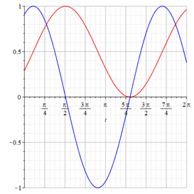
Equation (22) defines the Intensity as the volumetric power per unit area.

The Energy is plotted in red and the Intensity in blue. As energy is always positive, the Intensity it is not. It changes in time between the two maxima $\pm I_{max}$ . As it is a wave function, of course, is zero at some specific times.

We also note that the maximum Intensity (blue line) has a phase shift with respect to the maximum Energy of the electric field (red plot).

Intensity on a Sphere Area vs. Frequency and Distance

Replacing the values for $A$ (sphere of radius R) and in Eq. (22), we get:

$I=\frac{1}{4\pi R^2}\ 2\pi\varepsilon_0fE_{\max}^2\sin{\left[2(kx-\omega t)\right]}$

After simplifying, we get the expression of the Intensity on a sphere of radius R.

$I_{sphere}=\frac{E_{\max}^2}{{2R}^2}\varepsilon_0f\sin{\left[2(kx-\omega t)\right]}$ (23)

$\left[\frac{\frac{W}{m^3}}{m^2}\right]$ (23)

Recalling that $E_{rms}=\frac{E_{max}}{\sqrt2}$ , then we can write the equivalent equation as:

$I_{sphere}=\frac{E_{rms}^2}{R^2}\varepsilon_0f\sin{\left[2(kx-\omega t)\right]}$

$\left[\frac{\frac{W}{m^3}}{m^2}\right]$ (24)

This is the volumetric energy density distributed or spread in the whole sphere area.

Equation (24) tells us two important things: a) the energy of the wave is directly proportional to the frequency, i.e., the higher the frequency, the higher the energy; b) the energy decays with a factor $\frac{1}{R^2}$ .

Intensity on a Small Circular Area vs. Frequency and Distance

Let’s now take a small cap on the same sphere of radius R from the previous paragraph. By replacing the cap area (Eq. 15) and $\omega$ in Eq. (22), and taking $E_{rms}=\frac{E_{max}}{\sqrt2}$ , we obtain the Intensity at the cap area of the sphere.

$I_{cap}=\ \frac{1}{\frac{\pi}{4}\theta^2R^2}\ 2\pi\varepsilon_0{2E}_{rms}^2f\sin{\left[2(kx-\omega t)\right]}$

$I_{cap}=\ \frac{16}{\theta^2R^2}\varepsilon_0E_{rms}^2f\sin{\left[2(kx-\omega t)\right]}$

$\left[\frac{\frac{W}{m^3}}{m^2}\right]$ (25)

As we have seen in Eq. (17), the magnification factor is $F_\theta=\frac{16}{\theta^2}>400$ . Then, the intensity in this small area is much bigger than that of the full sphere area. That is:

$I_{cap}>\ 400\ I_{sphere}$

In Eq. (25) we see 3 variables affecting the intensity:

Frequency: the higher the frequency, the higher the energy.
Distance: the energy decays with a factor $\frac{1}{R^2}$
Aperture Angle: the smaller the cone angle between the source and the surface, the greater the intensity.

Intensity in Diffraction – The Phenomenon as Interference of Waves at Object Edges Explained

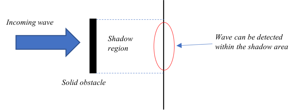
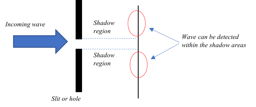
Waves generally tend to surround an obstacle by “wrapping” it in some way. The waves “bend” at the edges of an object and continue their path behind (to some degree), within the shadow area, making detection possible in that region. The obstacle could be solid/opaque or just a hole or slit.

$Intensity of Electromagnetic Waves in Diffraction from a Solid Object$

$Intensity of Electromagnetic Waves in Diffraction from a Slit or Hole$

Interference patterns behind the obstacle are classified as Near Field (Fresnel zone) and Far Field (Fraunhofer zone) and can be derived by using diffraction integrals.

My approach here is more general and based on my ideas of this phenomenon. I’ll demonstrate it easily by simply developing the interference of two waves.

If the obstacle does not totally absorb the wave energy, then the edges will produce retransmissions (reflections) of the incident wave on the obstacle edges in the form of spherical waves that will travel in many directions. Some front reflections in the opposite way will produce standing waves in front of the opaque parts of the obstacle. I’m interested in retransmissions that continue the direction of the incoming wave. Let’s analyze the slit interference.

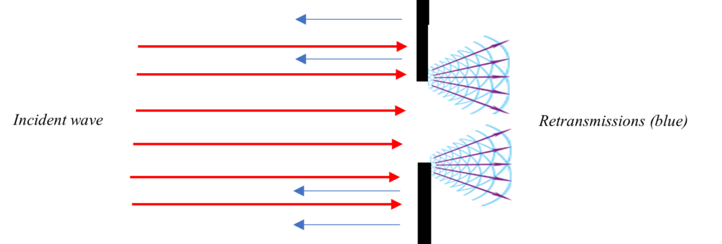
$Interference of Electromagnetic Waves in the Diffraction from a Slit or Hole$

I assume that the opaque edges of the obstacle do not absorb energy, so that the amplitude of the retransmitted wave remains almost the same as that of the incident wave.

I’ll analyze the slit interference by disregarding the fact that part of the incident wave might pass directly through the slit, by having a wave vector in the $x$ direction.

For simplicity, let’s consider just two retransmitted waves from both slit edges. I leave it to you to make the calculation of interference for the three waves, and in that case, see what happen.

Interference between two retransmitted waves from both slit edges

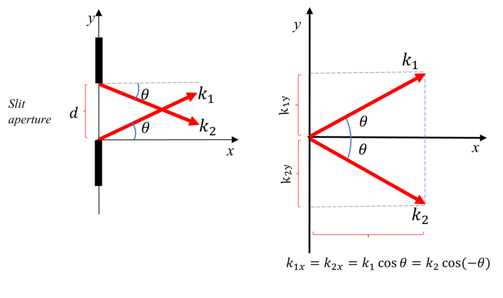
In this situation, the wave vectors are:

${\vec{k}}_1=k_{1x}\ \hat{i}+k_{1y}\ \hat{j}$	=>	$k_{1x}=k_1\cos{\theta}$ ;	$k_{1y}=k_1\sin{\theta}$
${\vec{k}}_2=k_{2x}\ \hat{i}+k_{2y}\ \hat{j}$	=>	$k_{2x}=k_2\cos{\left(-\theta\right)=k_2\cos{\theta}}$ ;	$k_{2y}=k_2\sin{\left(-\theta\right)=-k_2\sin{\theta}}$

The position vectors in this case are:

${\vec{r}}_1=x\ \hat{i}+y\ \hat{j}$

${\vec{r}}_2=x\ \hat{i}+(y-d)\ \hat{j}$

Wave Equation of Slit Interference

Let’s take the following superposition of the two waves, assuming the same amplitude and frequency:

$\varphi_{R(\vec{r},t)}=A\cos{({\vec{k}}_1{\vec{r}}_1-\omega t)}+A\cos{({\vec{k}}_2{\vec{r}}_2-\omega t)}$

To make it easy, let’s rename the arguments as:

$\propto=({\vec{k}}_1{\vec{r}}_1-\omega t)$ (25a)

$\beta=({\vec{k}}_2{\vec{r}}_2-\omega t)$ (25b)

The resulting wave can then be written in an easier way.

$\varphi_{R(\vec{r},t)}=A\left(\cos{\propto}+\cos{\beta}\right)=2A\cos{\left(\frac{\alpha+\beta}{2}\right)}\cos{\left(\frac{\alpha-\beta}{2}\right)}$ (26)

Now, let’s replace $\propto$ and $\beta$ as given in Eq. (25a) and (25b).

$\left(\frac{\alpha+\beta}{2}\right)=\frac{1}{2}\left({\vec{k}}_1{\vec{r}}_1-\omega t+{\vec{k}}_2{\vec{r}}_2-\omega t\right)=\frac{{\vec{k}}_1{\vec{r}}_1+{\vec{k}}_2{\vec{r}}_2}{2}-\omega t$

$\left(\frac{\alpha-\beta}{2}\right)=\frac{1}{2}\left({\vec{k}}_1{\vec{r}}_1-\omega t-{\vec{k}}_2{\vec{r}}_2+\omega t\right)=\frac{{\vec{k}}_1{\vec{r}}_1-{\vec{k}}_2{\vec{r}}_2}{2}$

If we plug in the above results in Eq. (26), we get the Wave Equation of Slit Interference:

$\varphi_{R(\vec{r},t)}=2A\cos{\left(\frac{{\vec{k}}_1{\vec{r}}_1-{\vec{k}}_2{\vec{r}}_2}{2}\right)}\cos{\left(\frac{{\vec{k}}_1{\vec{r}}_1+{\vec{k}}_2{\vec{r}}_2}{2}-\omega t\right)}$ (27)

Now let’s solve the dot products.

${\vec{k}}_1{\vec{r}}_1=\left(k_1\cos{\theta}\hat{i}+k_1\sin{\theta}\hat{j}\right)\ast\left(x\ \hat{i}+y\ \hat{j}\right)=k_1\cos{\theta}x+k_1\sin{\theta}y$

${\vec{k}}_2{\vec{r}}_2=\left(k_2\cos{\theta}\hat{i}-k_2\sin{\theta}\hat{j}\right)\ast\left[x\ \hat{i}+\left(y-d\right)\hat{j}\right]=k_2\cos{\theta}x-k_2\sin{\theta}(y-d)$

Since both waves have the same frequency, the wave vectors are also equal, $k_1=k_2=k$ .

${\vec{k}}_1{\vec{r}}_1=k(\cos{\theta}x+\sin{\theta}y)$

${\vec{k}}_2{\vec{r}}_2=k[\cos{\theta}x-\sin{\theta}\left(y-d\right)]$

Now we can proceed with the algebraic sum of the cosine arguments.

$\frac{{\vec{k}}_1{\vec{r}}_1+{\vec{k}}_2{\vec{r}}_2}{2}=\frac{k}{2}\left(\cos{\theta}x+\sin{\theta}y+\cos{\theta}x-\sin{\theta}y+\sin{\theta}d\right)=k\cos{\theta}x+\frac{kd\sin{\theta}}{2}$

$\frac{{\vec{k}}_1{\vec{r}}_1-{\vec{k}}_2{\vec{r}}_2}{2}=\frac{k}{2}\left(\cos{\theta}x+\sin{\theta}y-\cos{\theta}x+\sin{\theta}y-\sin{\theta}d\right)=k\sin{\theta}y-\frac{kd\sin{\theta}}{2}$

By replacing these results in Eq. (27), the wave equation of the slit interference becomes:

$\varphi_{R(\vec{r},t)}=2A\cos{\left(k\sin{\theta}y-\frac{kd\sin{\theta}}{2}\right)}\cos{\left(k\cos{\theta}x+\frac{kd\sin{\theta}}{2}-\omega t\right)}$ (28)

Where the arguments of the cosine functions represent the following:

$\Phi_1=k\sin{\theta}y-\frac{kd\sin{\theta}}{2}$	the spatial modulation in y-direction
$\Phi_2=k\cos{\theta}x+\frac{kd\sin{\theta}}{2}-\omega t$	the wave propagating in x-direction

Let’s freeze the time and take a snapshot of the resulting wave at any time, say $t=0$ . Constructive interference happens when cosines are maximum, i.e., at $n\pi$ ( $n=0,\pm1,\pm2\ldots$ ). In this case, the arguments can be written as:

$\Phi_1=k\sin{\theta}y-\frac{kd\sin{\theta}}{2}=n\pi$ (29)

$\Phi_2=k\cos{\theta}x+\frac{kd\sin{\theta}}{2}=n\pi$ (30)

Since we are interested in the interference fringes in the y-z plane, let’s analyze $\Phi_1$ .

$\sin{\theta}y-\frac{d\sin{\theta}}{2}=\frac{n\pi}{k}$	=>	$\sin{\theta}y=\frac{n\pi}{k}+\frac{d\sin{\theta}}{2}$
$y=\frac{n\pi}{k\sin{\theta}}+\frac{d}{2}=\frac{n\pi\lambda}{2\pi\sin{\theta}}+\frac{d}{2}$	=>	$(y-\frac{d}{2})=\frac{\pmn\lambda}{2\sin{\theta}}$

The last equation tells us that the interference pattern is centered at $y=\frac{d}{2}$ .

If we make $y=0$ , we get the famous equation of slit interference based on the experiment made by Young, where we can calculate the location of the bright bands on a screen in the y-z plane, placed at a distance $x\ggd$ from the slit. That is,

$d\sin{\theta}=\mpn\lambda$

( $n=0,\mp1,\mp2\ldots$ )

constructive interference bands of a slit

Here, $\theta$ is half the angle between any two chosen wave vectors which originate at the slit. It is not arbitrary, but perfectly defined.

In the physics books and literature out there, $\theta$ is the angle of an arbitrary line traced from the slit to the screen to explain that the path difference between the two waves is the cause of the interference. Even when this is true, you will never know what is happening and why.

I have assumed symmetrical angles for the wave vectors. What happens if the angle between the wave vectors is different?

The result will be the same. What matters is the relative angle between the wave vectors, not the individual angles. In our case, the relative angle is $2\theta$ , but $\theta$ can be the sum of two different angles.

Now let’s find the equation of the wave fronts from the resulting interference. We can equal Eq. (29) and Eq. (30) to obtain a function y=f(x) that we can plot in order to see the shape of the wave fronts.

$k\sin{\theta}y-\frac{kd\sin{\theta}}{2}=k\cos{\theta}x+\frac{kd\sin{\theta}}{2}$
$\sin{\theta}y=\cos{\theta}x+\frac{dsin(\theta)}{2}$	=>	$y=\frac{x}{\tan{\theta}}+\frac{d}{2}$

By replacing $\tan{\theta}=\frac{y}{x}$ and rearranging, we get the following equation that describes the pattern formed by the wave fronts:

$y^2-\frac{d}{2}y-x^2=0$

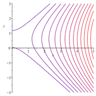
The figure shows some lines of the wave fronts for a slit width = 2.42 units of length. If we put a screen perpendicular to this page, say at x=4, we will see that the wave reaches areas that are well beyond the shadow regions of the slit.

Conclusions

This study clearly demonstrates the dependence of the wave energy propagation not only as a function of an area, but more generally, as a function of three variables, such as frequency, distance, and aperture angle from the source. The wave equation obtained in the analysis agrees with the Planck’s formula.

Volumetric Power and Intensity are defined in order to account for a correct energy distribution of EMW in space. The Intensity wave equation is derived, showing the relationship with the source’s frequency, distance, and aperture angle.

The Intensity in Diffraction is demonstrated as an interference phenomenon. The wave equation of the slit interference is deduced, from which the interference pattern is obtained in complete agreement with the Young experiment.

Bibliography

M. Muhibbullah et al, “Frequency dependent power and energy flux density equations of the electromagnetic wave” (2017), Results in Physics 7 (2017) 435–439. https://www.sciencedirect.com/science/article/pii/S2211379716302170?via%3Dihub
Johan Sjöholm and Kristoffer Palmer, “Angular Momentum of Electromagnetic Radiation” (2007), Uppsala School of Engineering and Department of Astronomy and Space Physics. https://arxiv.org/ftp/arxiv/papers/0905/0905.0190.pdf
Kirk T. McDonald, “Does Destructive Interference Destroy Energy?” (2014, 2018), Princeton University. https://www.physics.princeton.edu/~mcdonald/examples/destructive.pdf
Schantz HG., 2018 “Energy velocity and reactive fields” (2018), Phil. Trans. R. Soc. A 376: 20170453. http://dx.doi.org/10.1098/rsta.2017.0453
David Morin, “Interference and diffraction” (2010), Harvard. https://scholar.harvard.edu/files/david-morin/files/waves_interference.pdf
Gerhard Kristensson, “Spherical vector waves” (2014). https://www.eit.lth.se/fileadmin/eit/courses/eit080f/Literature/book.pdf

Physics Answers