Raul Fattore
April 7, 2023
The present study is divided into six parts
Part-1 Part-2 Part-3 Part-5 Part-6
Table of Contents
In This Paper
Following the analysis made in Part-3, the second external force is evaluated in this study.
The nuclear response to external forces is analyzed with the aim to observe any changes in the nuclear mass and study the behavior of the refractive index under such changes.
The analysis will be performed in the time domain as well as in the frequency domain by means of the Fast Fourier Transform (FFT) method. The external forces applied to the nucleus were classified into three types:
- The force originated by a polarized transverse electromagnetic wave (TEM) (see Part-3)
- The force originated by a polarized TEM plus a static electric field
- The force originated by a signal plus a static electric field (see Part-5)
Abstract
Some efforts have been made to prove negative mass behavior through some experiments performed in mechanics [1], and other disciplines [9], as well as some theories in electrostatics [2,3,4,5,6,7,8], but I haven’t found research about similar effects at the atomic level, where the most elementary mass given by the atomic nucleus is to be found.
- Is the second Newton’s law still valid with negative mass?
- What could happen if we make the atom behave in a negative mass regime?
- Is the negative refractive index related to negative mass?
- Are we able to control the magnitude of mass?
- Are we able to control the sign of mass?
The answers to these questions are given through this series of papers, with results that are coincident with experimental data, except for the negative mass regime. Experiments must be done to confirm or invalidate the theory developed in these articles. Needless to say, if experiments validate this theory, then a significant change in mankind is going to happen. In that case, I strongly ask scientists to cooperate by making use of the derived technologies for good and refrain from doing it for evil.
Introduction
The theory presented in these papers, as described in Part-1, is based on three fundamental aspects that have proved to be extremely effective to describe physical phenomena and predicting results that agree with experimental data [10, 11, 12]:
• Spinning Ring Model of Elementary Particles (toroidal ring of continuous charge)
• New Atomic Model
• The Universal Electrodynamic Force
Based on the new atomic model, a shell arrangement of the nuclear particles has been assumed in Part 1, as shown in Fig. 1.
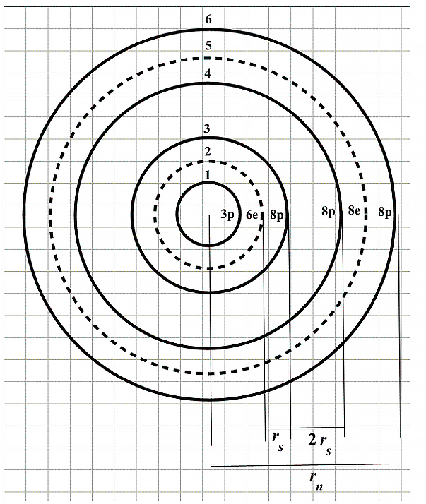
Assumed shell arrangement for Aluminum atomic nucleus
This sandwich configuration keeps the particles very tightly bound together. Note that at three shells in from the outermost shell, there are always two proton shells in a row for the larger nuclides.
This weak binding allows the outermost sandwich of shells to have liquid-like properties and forms the proper justification for a Liquid Drop Model of the nucleus.
As we already know, the torus ring model of the particles has an associated electric field as well as a magnetic field. However, due to the very tight packing configuration of the particles, we may safely assume that the distance among shells is extremely tiny and that the predominant force in the nucleus is of electrostatic origin, while the weaker magnetic forces will add some contribution to the equilibrium distance between each shell. As demonstrated in Part 1, mass is an intrinsic property of the atomic nucleus. Under natural circumstances, it has a constant universal magnitude and is always positive. However, with some proper external agents, we might be able to manipulate the intrinsic mass by changing its magnitude and sign.
II. Nuclear Response to Force Caused by a Polarized Transverse Electromagnetic Wave (TEM) plus a Static Electric Field
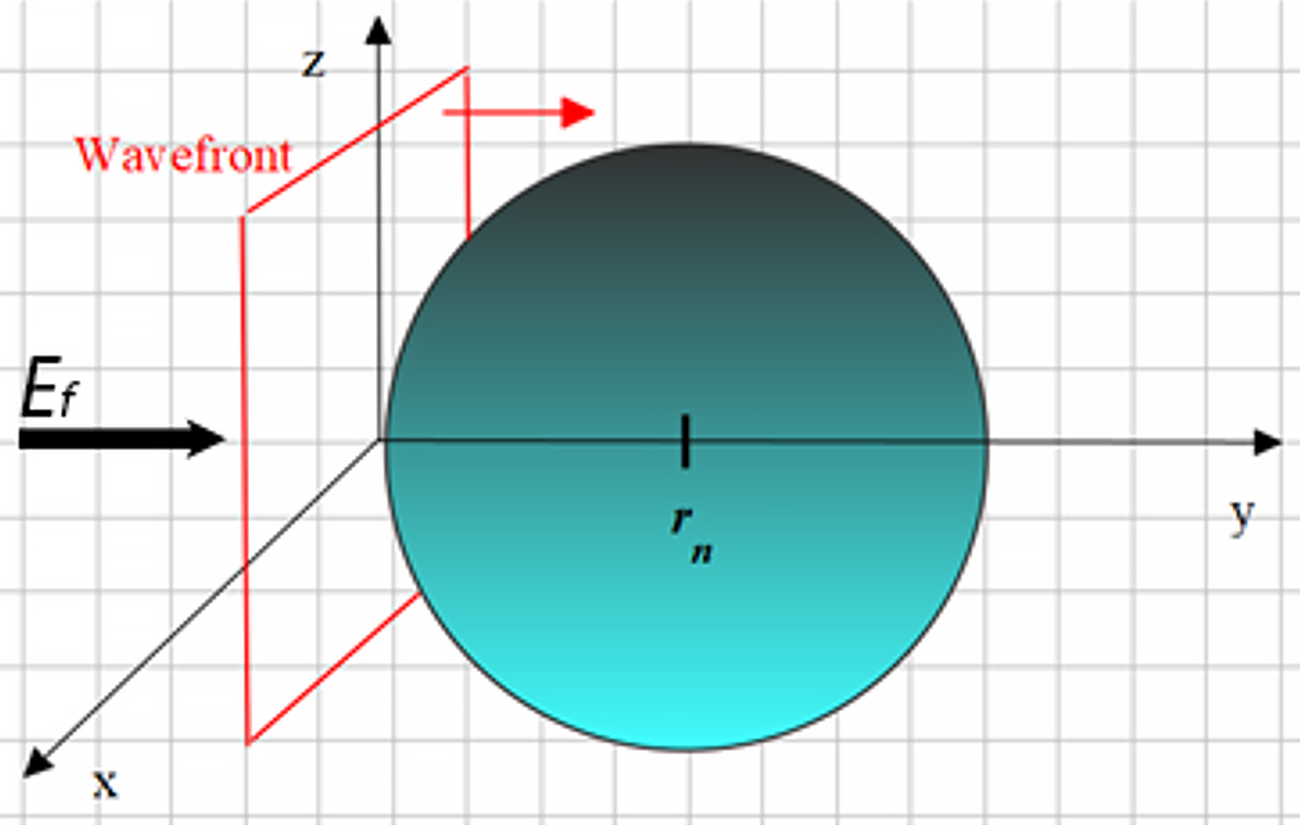
External wavefront and static electric field acting on the nucleus
Assume that a plane wave of amplitude E_m, frequency \omega, and propagation velocity c in the y-direction strikes the outer shell of the “nuclear sphere”.
Assume also that we add a static electric field that is parallel to the y-z plane in the y-direction. The components of the fields in cartesian coordinates are: {\vec{E}}_f=0\hat{i}+E_f\hat{j}+0\hat{k}, and in spherical coordinates we have,
{\vec{E}}_f=E_fsin\left(\theta\right)sin\left(\phi\right)\hat{r}+E_fsin\left(\phi\right)cos\left(\theta\right)\hat{\theta}+E_fcos\left(\phi\right)\hat{\phi}
As the static electric field is parallel to the y-z plane, and pointing in the y direction, \emptyset=\frac{\pi}{2} and \theta=\frac{\pi}{2}. Then, the expression of the electric field is
{\vec{E}}_f=E_f\hat{r} (a)
As this static field is added to the wave, the composed electric field E “seen” by the nucleus will have a constant value given by E_f plus the component of the oscillating electric field corresponding to the wave.
We disregard some minor scattering caused by the few outer electrons in the atom, which are located at a very long distance from the nucleus. The incident wave energy may be totally absorbed, partially absorbed, or not absorbed at all by the nuclear shells.
The momentum density of any wave in vacuum is given by: \frac{dp}{dV}=\frac{EB}{\mu_0c^2}. By replacing B=\frac{E}{c}, we get \frac{dp}{dV}=\frac{E^2}{\mu_0cc^2}, which, by replacing c^2 gives \frac{dp}{dV}=\frac{\mu_0\varepsilon_0E^2}{\mu_0c}, so that the momentum density in function of only one of the EM fields is: \frac{dp}{dV}=\frac{\varepsilon_0E^2}{c}\left[\frac{Ns}{m^3}\right]. Recall that we can write the force as the change in momentum, i.e., F=\frac{dp}{dt}, so we can write the momentum density as the force exerted by the wave on the nucleus volume: \frac{dp}{dV}\cdot\frac{dt}{dt}=\frac{\varepsilon_0E^2}{c}, which gives us
Fdt=\frac{\varepsilon_0E^2}{c}dV (1)
Where:
dt: time needed by the wave to travel with velocity c (or v) across the nucleus diameter (2\ r_n) from t=0 to t=\frac{2r_n}{c} (or t=2\frac{r_n}{v}). Calculations will be made for a wave velocity of c and v in the nucleus.
dV: the volume element for the spherical nucleus (r^2\sin{\left(\theta\right)}drd\theta\ d\emptyset).
Note that the force given by (1) is calculated in vacuum and contains the vacuum permittivity \varepsilon_0. We ignore the value of the nuclear permittivity of Aluminum. Therefore, the same permittivity will be used for further calculations to be consistent with the Coulomb Force and the Universal Force used in the study.
The polarized wave acting on the nucleus is given by Eq. (21) and (22) in Part-2, whose magnitude is repeated here:
E\left(r,t\right)=E_m\cos{\left(Kr-\omega t\right)} (2)
The total external field acting on the nucleus is given by
E=E_f+E_mcos\left(Kr-\omega t\right) (2a)
We assume that the outer shell of the “nuclear sphere” is reached by a plane wavefront traveling in the -direction with velocity c at t=0. That is, the origin of coordinates is taken at the incident edge of the nucleus, which means the nucleus center is shifted (r-r_n).
To calculate the exerted force on the atomic nucleus, we need to integrate the total field given by Eq. (1). Considering that the force is constant on the time interval, the force integrated on the nucleus volume is:
F\int_{0}^{t}dt=\int_{0}^{2\pi}\int_{0}^{\pi}\int_{0}^{r_n}{\frac{\varepsilon_0E^2}{c}\left(r-r_n\right)^2}dr\ d\theta\ d\phi (3)
Defining the time interval for the force integral
How to determine the time interval for integration? Three possibilities have been chosen that might give us a kind of “average force” (though is not an average) on the nuclear volume:
- The wave’s travel time through the nucleus for wave velocity v_w, that is t=2\frac{r_n}{v_w} (absorption)
- The wave’s travel time through the nucleus for wave velocity c, that is t=2\frac{r_n}{c} (transmission)
- The wave period, that is t=T=\frac{2\pi}{\omega} (absorption/ transmission, depends on wave vector’s choice)
1. Integrating the force caused by the electric field and the wave, for nuclear travel time, with wave velocity “vw”
Replacing the wave Eq. (2) into the integral (3), and setting the time interval for this case,
F\int_{0}^{\frac{2r_n}{v_w}}dt=\frac{\varepsilon_0}{c}\int_{0}^{2\pi}{\int_{0}^{\pi}{\int_{0}^{r_n}{\left(E_f+E_mcos\left(Kr-\omega t\right)\right)^2\left(r-r_n\right)^2\sin{\left(\theta\right)}d}r}d}\theta d\emptyset
After integrating and doing some algebra, we get the expression of the wave force on the nucleus for this case:
F_{ext}=\frac{2\pi\varepsilon_0v_w}{3c K^3r_n}\cdot\left(-\frac{3E_m^2\sin{\left(2Kr_n-2\omega t\right)}}{8}-12E_fE_m\sin{\left(Kr_n-\omega t\right)}+\frac{3E_m^2\left(K^2r_n^2-\frac{1}{2}\right)\sin{\left(2\omega t\right)}}{4}+\frac{3E_m^2r_nK\cos{\left(2\omega t\right)}}{4}+6E_fE_m\left(K^2r_n^2-2\right)\sin{\left(\omega t\right)}+r_n\left(12E_fE_m\cos{\left(\omega t\right)}+K^2r_n^2\left(E_f^2+\frac{E_m^2}{2}\right)\right)K\right) (4)
2. Integrating the force caused by the electric field and the wave, for nuclear travel time, with wave velocity “c”
Replacing the wave Eq. (2) into the integral (3), and setting the time interval for this case,
F\int_{0}^{\frac{2r_n}{c}}dt=\frac{\varepsilon_0}{c}\int_{0}^{2\pi}{\int_{0}^{\pi}{\int_{0}^{r_n}{\left(E_f+E_mcos\left(Kr-\omega t\right)\right)^2\left(r-r_n\right)^2\sin{\left(\theta\right)}d}r}d}\theta\ d\emptyset
After integrating and doing some algebra, we get the expression of the wave force on the nucleus for this case:
F_{ext}=\frac{\pi\varepsilon_0}{6K^3r_n}\cdot\left(4E_f^2K^3r_n^3+2E_m^2K^3r_n^3+6E_m^2K^2\sin{\left(\omega t\right)}\cos{\left(\omega t\right)}r_n^2+24E_fE_mr_n^2\sin{\left(\omega t\right)}K^2+6E_m^2K\sin^2{\left(r_nK-\omega t\right)}r_n+6E_m^2K\cos^2{\left(r_nK-\omega t\right)}r_n-6E_m^2K\sin^2{\left(\omega t\right)}r_n-6E_m^2\sin^2{\left(r_nK-\omega t\right)}\omega t-6E_m^2\cos^2{\left(r_nK-\omega t\right)}\omega t+6E_m^2\sin^2{\left(\omega t\right)}\omega t+6E_m^2\cos^2{\left(\omega t\right)}\omega t+48E_fE_mK\cos{\left(\omega t\right)}r_n-3E_m^2r_nK-3E_m^2\sin{\left(r_nK-\omega t\right)}\cos{\left(r_nK-\omega t\right)}-3E_m^2\sin{\left(\omega t\right)}\cos{\left(\omega t\right)}-48E_fE_m\sin{\left(r_nK-\omega t\right)}-48E_fE_m\sin{\left(\omega t\right)}\right) (5)
3. Integrating the force caused by the electric field and the wave, for a wave period
Replacing the wave Eq. (2) into the integral (3), and setting the time interval for this case,
F\int_{0}^{\frac{2\pi}{\omega}}dt=\frac{\varepsilon_0}{c}\int_{0}^{2\pi}{\int_{0}^{\pi}{\int_{0}^{r_n}{\left(E_f+E_mcos\left(Kr-\omega t\right)\right)^2\left(r-r_n\right)^2\sin{\left(\theta\right)}d}r}d}\theta\ d\emptyset
After integrating and doing some algebra, we get the expression of the wave force on the nucleus for this case:
F_{ext}=\frac{2\varepsilon_0\omega}{3c K^3}\cdot\left(-\frac{3E_m^2\sin{\left(2Kr_n-2\omega t\right)}}{8}-12E_fE_m\sin{\left(Kr_n-\omega t\right)}+\frac{3\left(K^2r_n^2-\frac{1}{2}\right)E_m^2\sin{\left(2\omega t\right)}}{4}+\frac{3E_m^2r_nK\cos{\left(2\omega t\right)}}{4}+6E_fE_m\left(K^2r_n^2-2\right)\sin{\left(\omega t\right)}+r_n\left(12E_fE_m\cos{\left(\omega t\right)}+K^2r_n^2\left(E_f^2+\frac{E_m^2}{2}\right)\right)K\right) (6)
Now that we have the three versions of the external force exerted on the nucleus by a polarized TEM plus a static electric field, it’s time to evaluate the nuclear response related to mass and refractive index behaviors.
II.a Nuclear Mass Analysis due to Force caused by Static Field plus Wave (4) – Partial or Total Energy Absorption
The intrinsic net force in the nucleus was already defined with Eq. (23) in Part-1. Now we have the action of an external force acting on the nucleus that will interact with the internal force. By applying Newton’s second law, we have
\sum F=m_n\cdot a_{ep}=F_{net}+F_{ext} => m_n\cdot a_{ep}=F_{net}+F_{ext}
m_n=\frac{1}{a_{ep}}\cdot\left(F_{net}+F_{ext}\right) (7)
By replacing the forces in (7), we obtain the expression of the nuclear mass for this case:
m_n=\frac{1}{a_{ep}\left(t\right)}\cdot\left(-\frac{{3.410}^{12}\cdot q^2\left(1-\frac{v_{ep}^2\left(t\right)}{c^2}+\frac{v_{ep}^2\left(t\right)r_{ep}\left(t\right)a_{ep}\left(t\right)}{c^4}+\frac{v_{ep}^4\left(t\right)}{c^4}+\frac{2r_{ep}\left(t\right)a_{ep}\left(t\right)}{c^2}\right)}{r_{ep}^2\left(t\right)}+\frac{{2.0510}^{13}\cdot q^2}{r_n^2}+\frac{2\pi\varepsilon_0v_w}{3c K^3r_n}\cdot\left(-\frac{3E_m^2\sin{\left(2Kr_n-2\omega t\right)}}{8}-12E_fE_m\sin{\left(Kr_n-\omega t\right)}+\frac{3E_m^2\left(K^2r_n^2-\frac{1}{2}\right)\sin{\left(2\omega t\right)}}{4}+\frac{3E_m^2r_nK\cos{\left(2\omega t\right)}}{4}+6E_fE_m\left(K^2r_n^2-2\right)\sin{\left(\omega t\right)}+r_n\left(12E_fE_m\cos{\left(\omega t\right)}+K^2r_n^2\left(E_f^2+\frac{E_m^2}{2}\right)\right)K\right)\right) (8)
Recall that:
r_{ep}\left(t\right)=\left(0.37r_n+A_e\cos{\left(\omega_et\right)}-A_p\cos{\left(\omega_pt\right)}\right);
v_{ep}\left(t\right)=\left(-A_e\omega_e\sin{\left(\omega_et\right)}+A_p\sin{\left(\omega_pt\right)}\omega_p\right);
a_{ep}\left(t\right)=\left(-A_e\omega_e^2\cos{\left(\omega_et\right)}+A_p\omega_p^2\cos{\left(\omega_pt\right)}\right)
Some graphs as examples are shown below to have a perception of what could be done to modify the nuclear mass magnitude and sign.
The main parameters used for the net force are:
r_n=3.5\ {10}^{-15}\ [m]; A_e=2\ {10}^{-16}\ [m]; A_p={10}^{-3}A_e\ [m]; N_0=378; N_s=312
\omega_e={10}^{15}\ [\frac{1}{s}]; \omega_p={10}^{16}\ [\frac{1}{s}]
While for the wave: v_w=v_{ep}\left(t\right); K=\frac{\omega}{v_{ep}\left(t\right)}
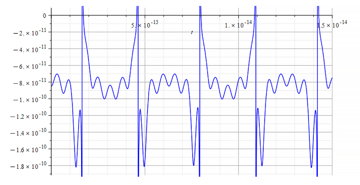
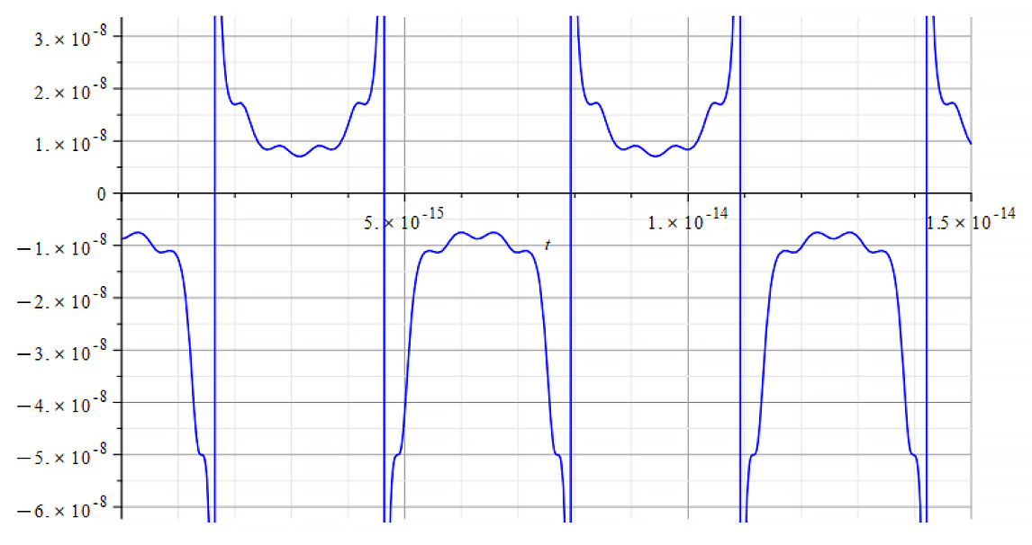
Time Analysis of the Nuclear Mass
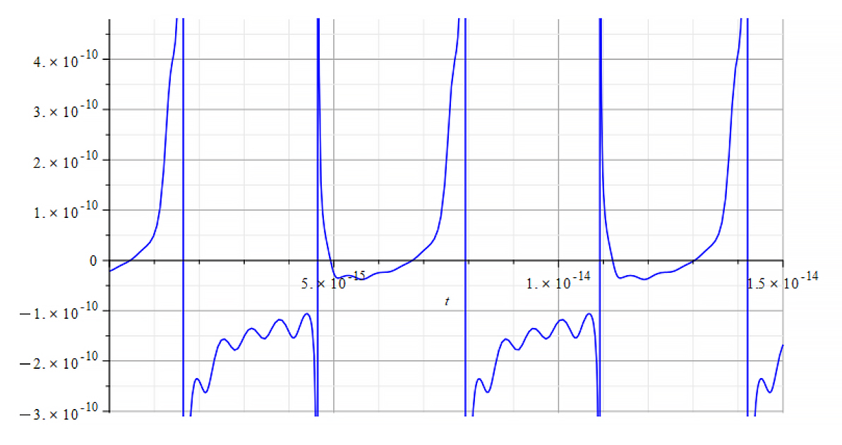 |  |
| +{E}_{f} Mass vs. time for the following parameters: \omega={10}^{12}\ [\frac{1}{s}]; E_m={10}^{26}\ [\frac{V}{m}]; E_f={10}^{26}\ [\frac{V}{m}] | -{E}_{f} Mass vs. time for the following parameters: \omega={10}^{12}\ [\frac{1}{s}]; E_m={10}^{26}\ [\frac{V}{m}]; E_f={-10}^{26}\ [\frac{V}{m}] |
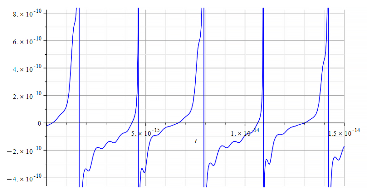 | 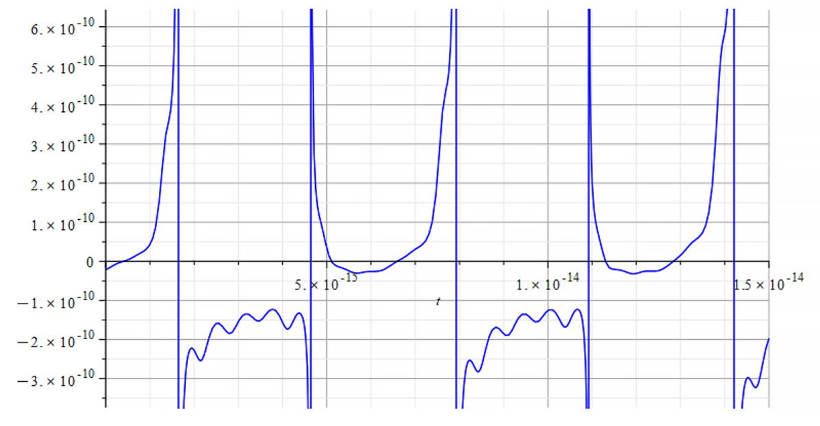 |
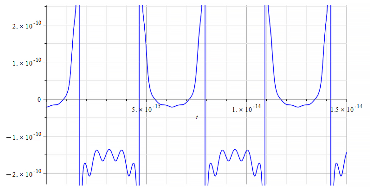
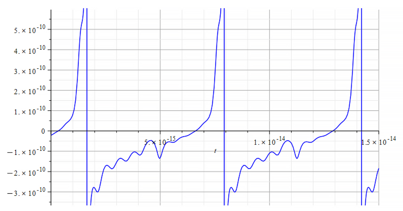
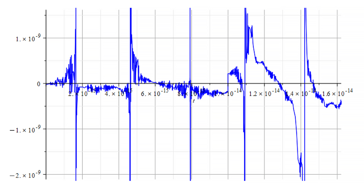
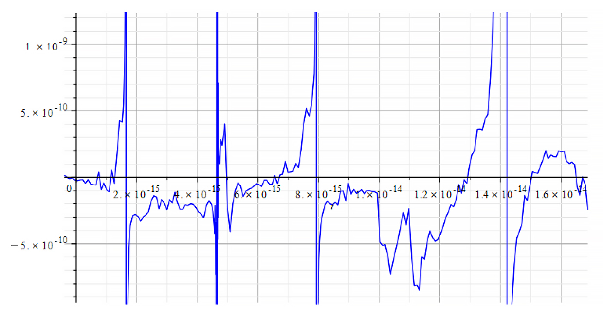
| +{E}_{f} Mass vs. time for the following parameters: \omega={10}^{14}\ [\frac{1}{s}]; E_m={10}^{26}\ [\frac{V}{m}]; E_f={2.5\ 10}^{26}\ [\frac{V}{m}] | -{E}_{f} Mass vs. time for the following parameters: \omega={10}^{14}\ [\frac{1}{s}]; E_m={10}^{26}\ [\frac{V}{m}]; E_f={-2.5\ 10}^{26}\ [\frac{V}{m}] |
 | |
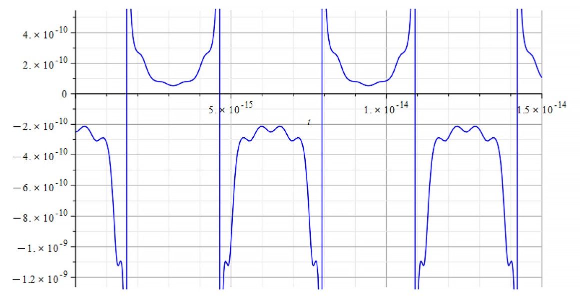
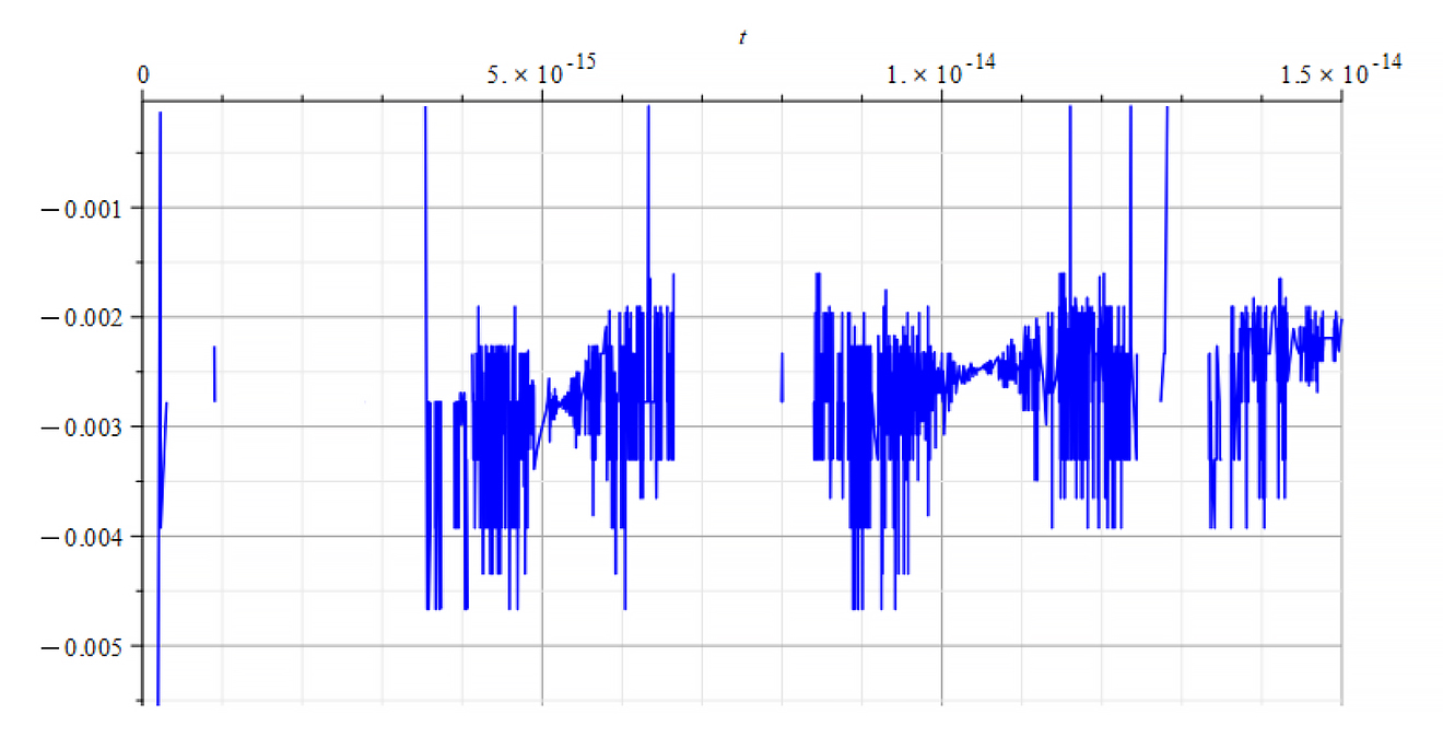
| +{E}_{f} Mass vs. time for the following parameters: \omega={10}^{17}\ [\frac{1}{s}]; E_m={10}^{26}\ [\frac{V}{m}];E_f={\pm2.5\ 10}^5\ [\frac{V}{m}] | -{E}_{f} Same result for both polarities |
From the period of the mass plot, we determine that the oscillation frequency is approximately:
f=1.6\ {10}^{14}\ [Hz]
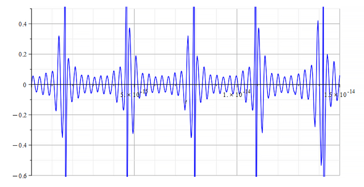
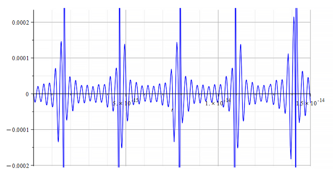
Frequency Analysis of the Nuclear Mass with FFT
Total number of samples N=2^{15}, sampling frequency f_s=2^3\ f_w (wave frequency), which gives a frequency resolution \Delta_{f}=\frac{f_s}{N}[Hz] and a total acquisition time of T=\frac{N}{f_s}[s]. The frequency at the i-sample number on the plot is determined by f=\frac{N_{(i)}}{T}\ [Hz].
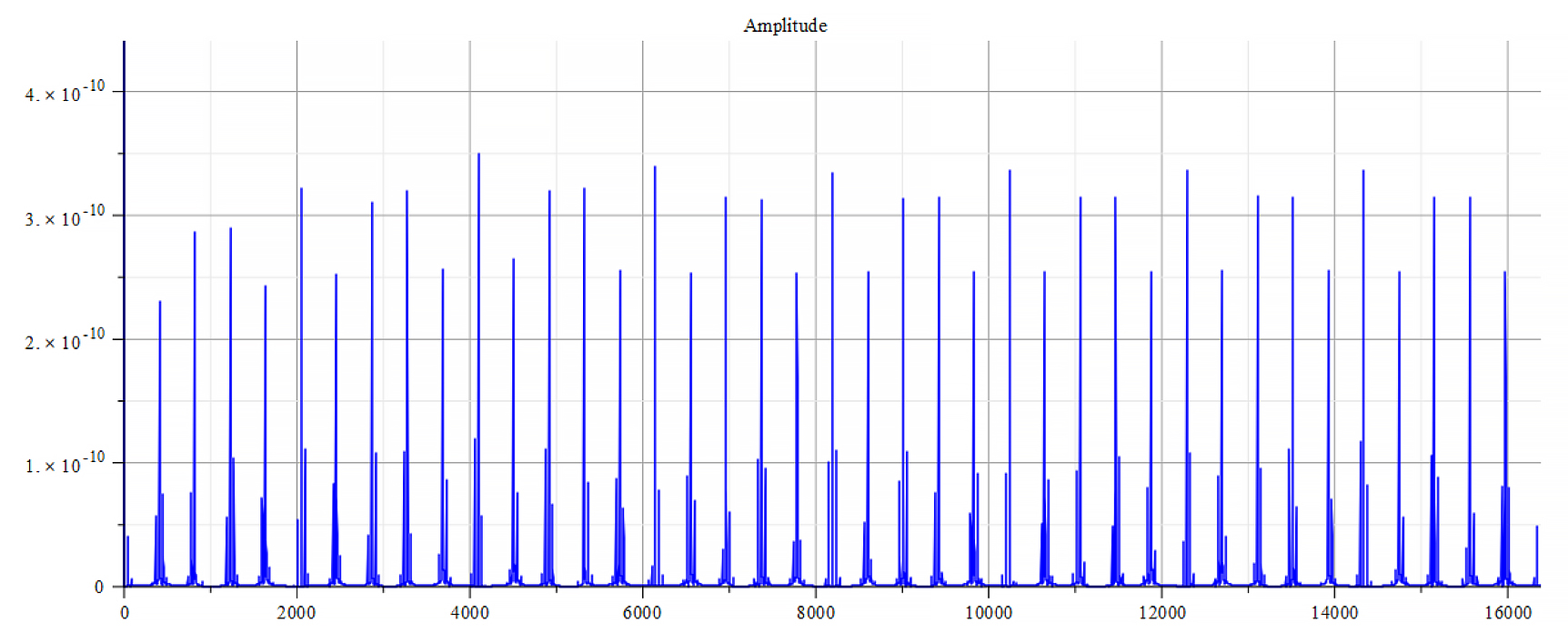
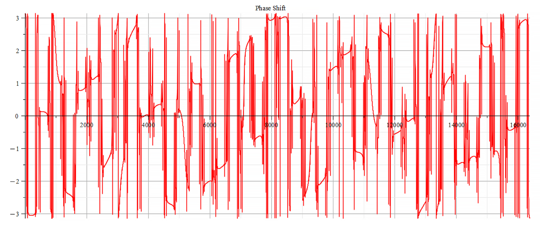
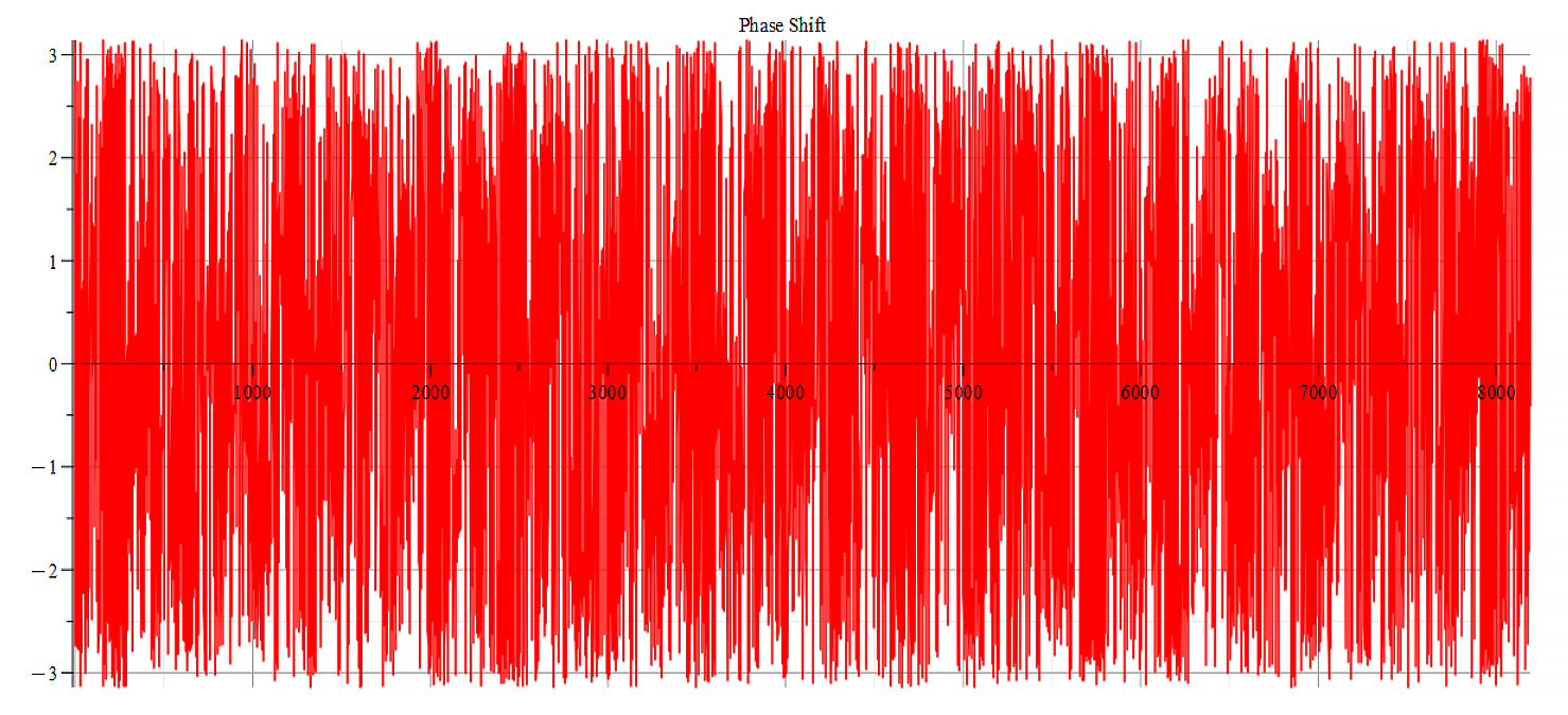
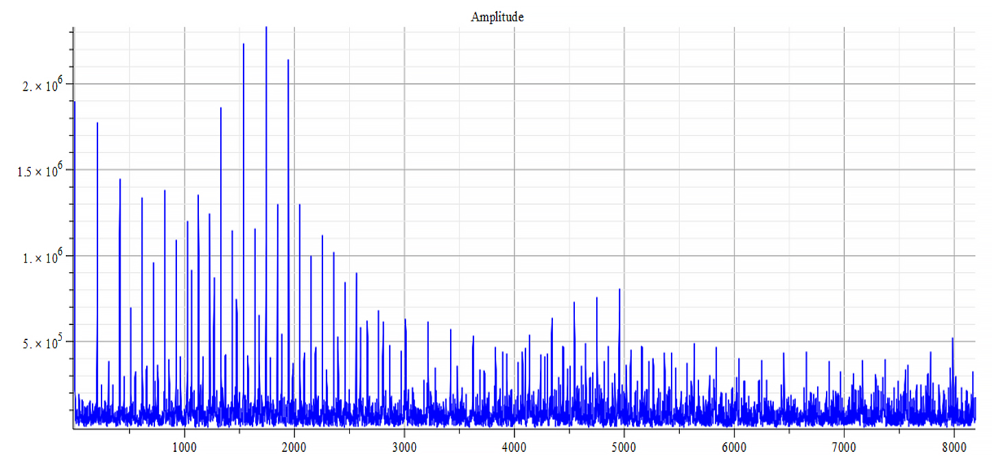
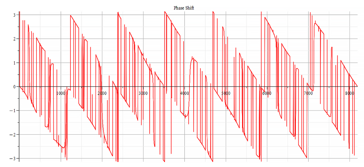
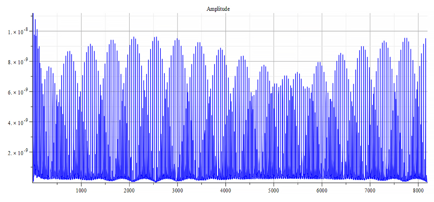
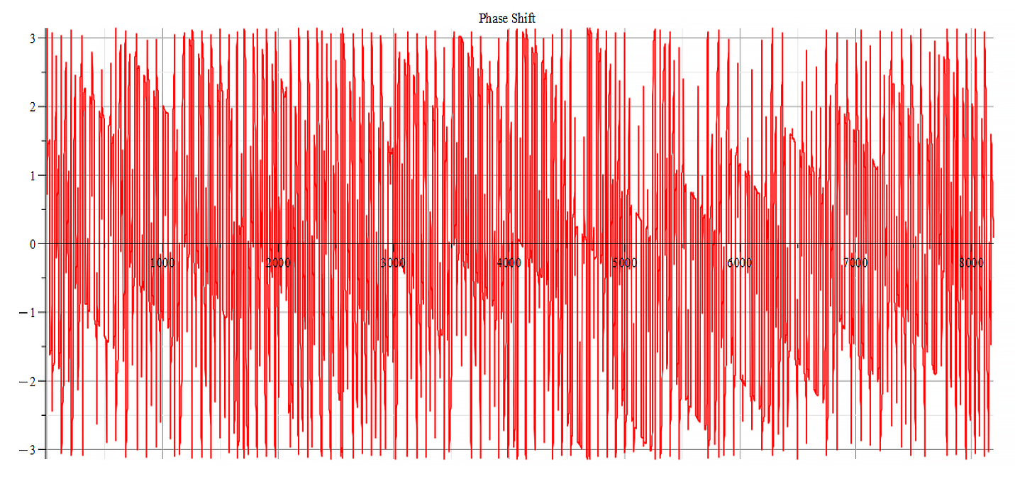
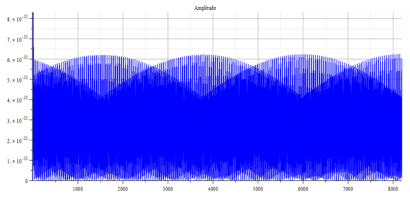
For +Ef
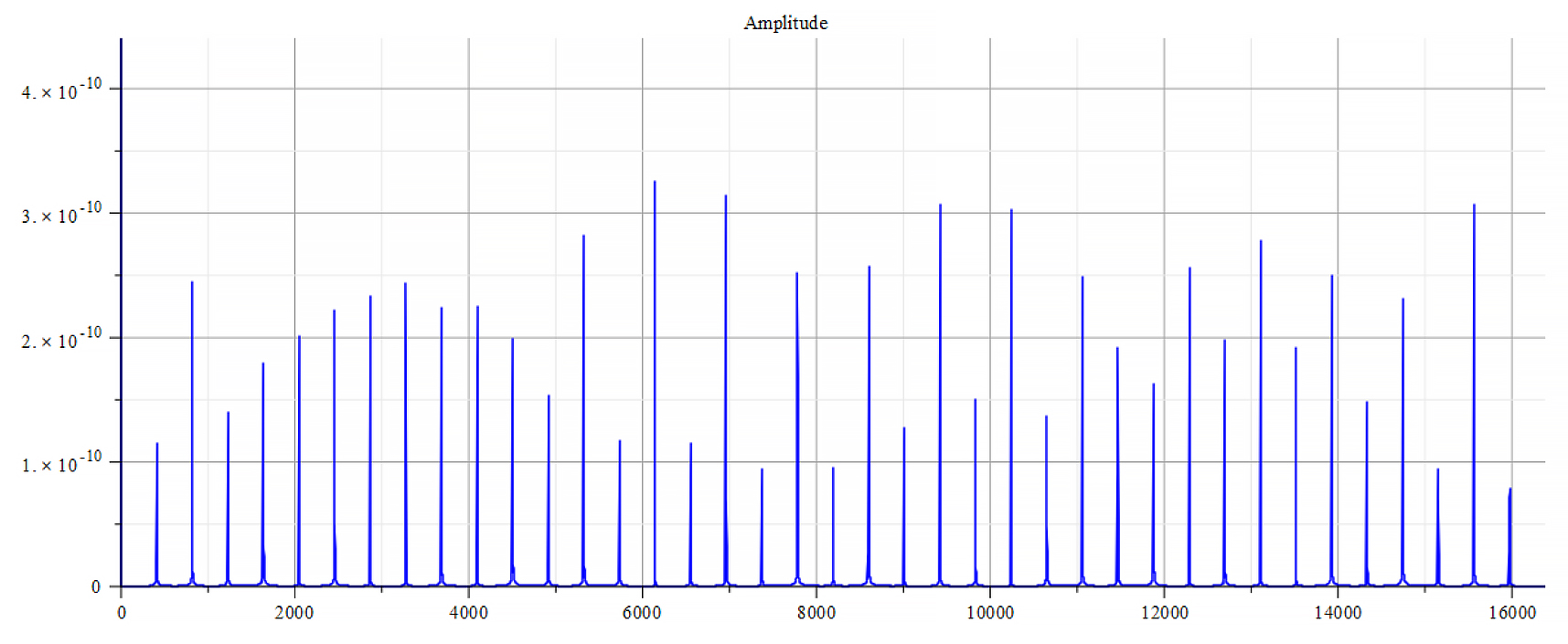
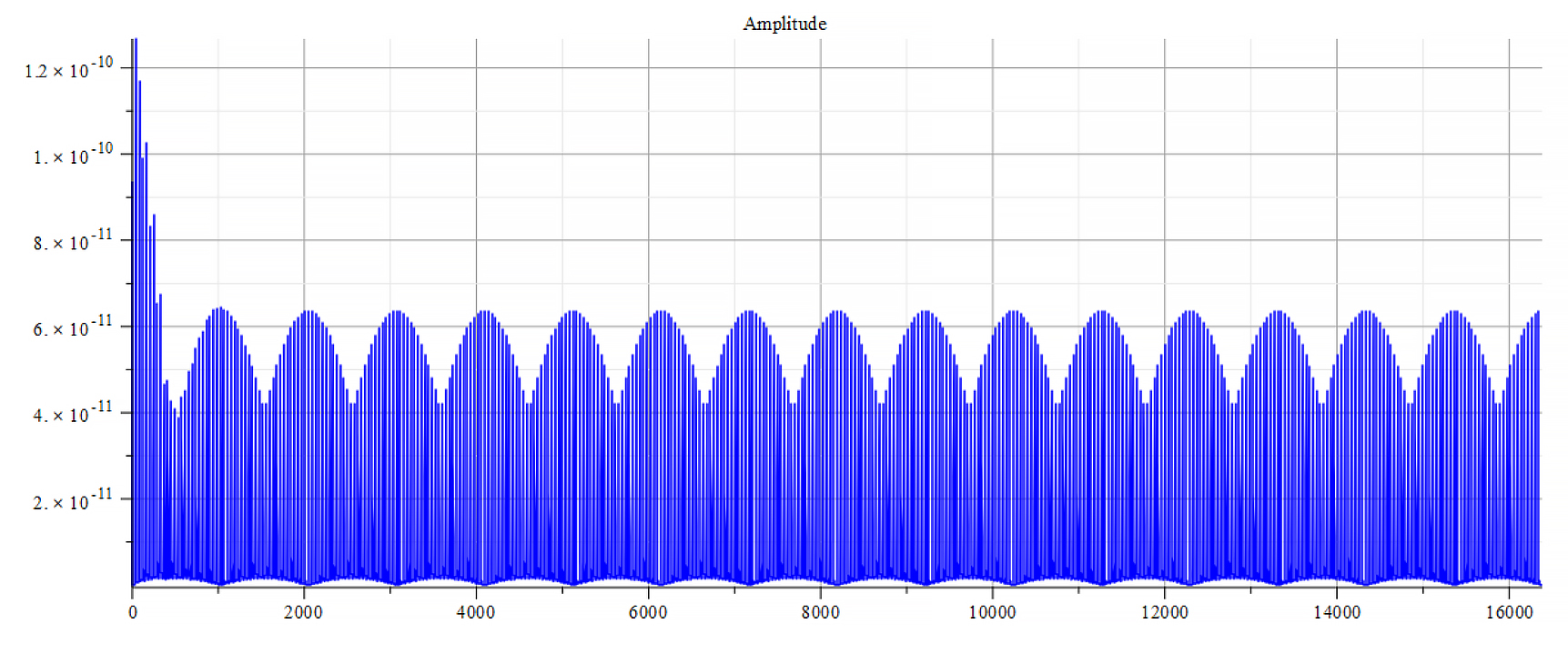
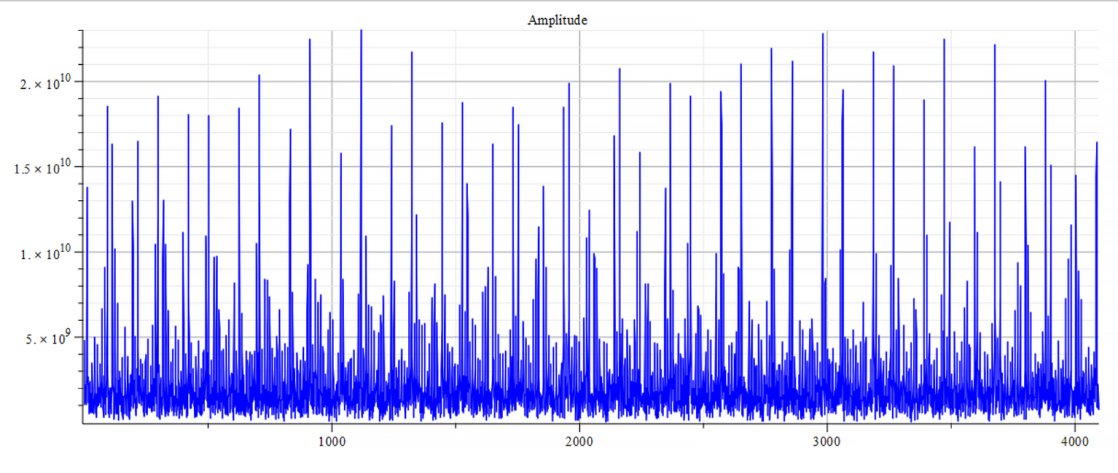
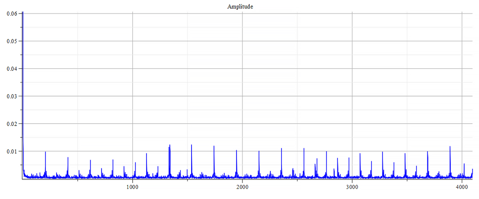
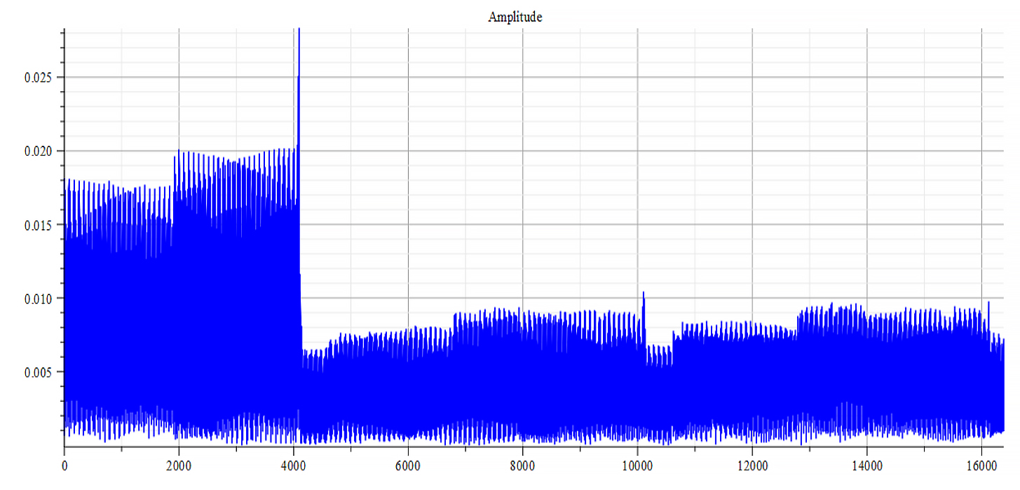
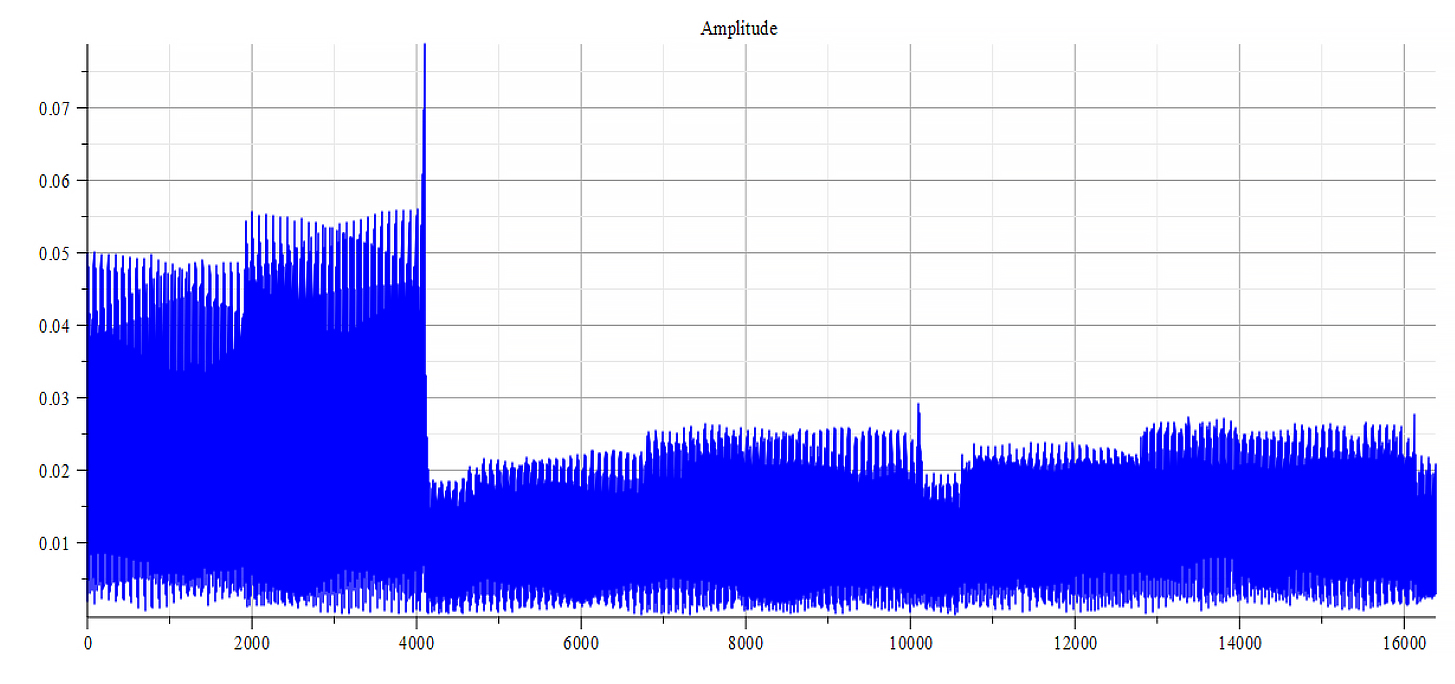
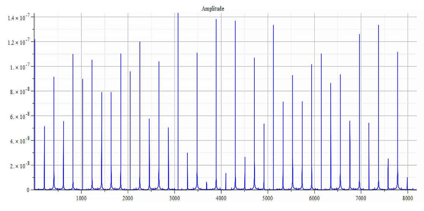
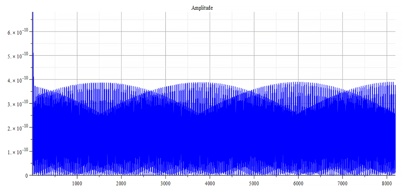
Frequency spectrum for the following parameters: \omega={10}^{12}\ [\frac{1}{s}]; E_m={10}^{26}\ [\frac{V}{m}]; E_f={10}^{26}\ [\frac{V}{m}]
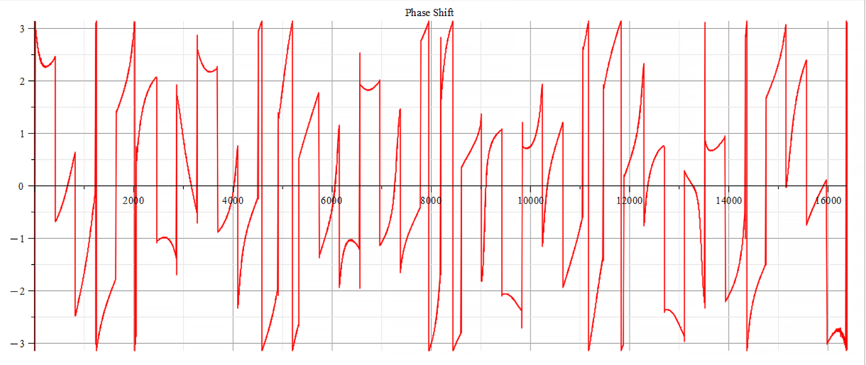
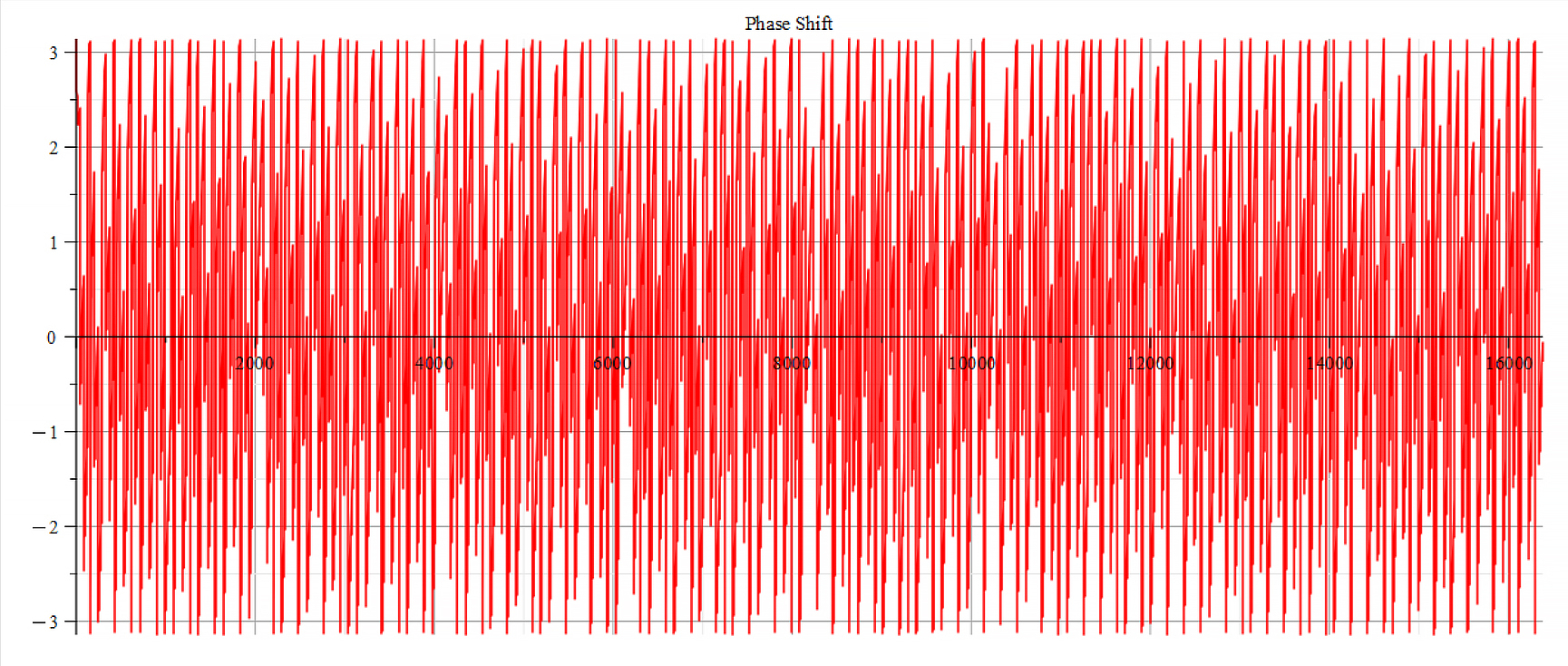
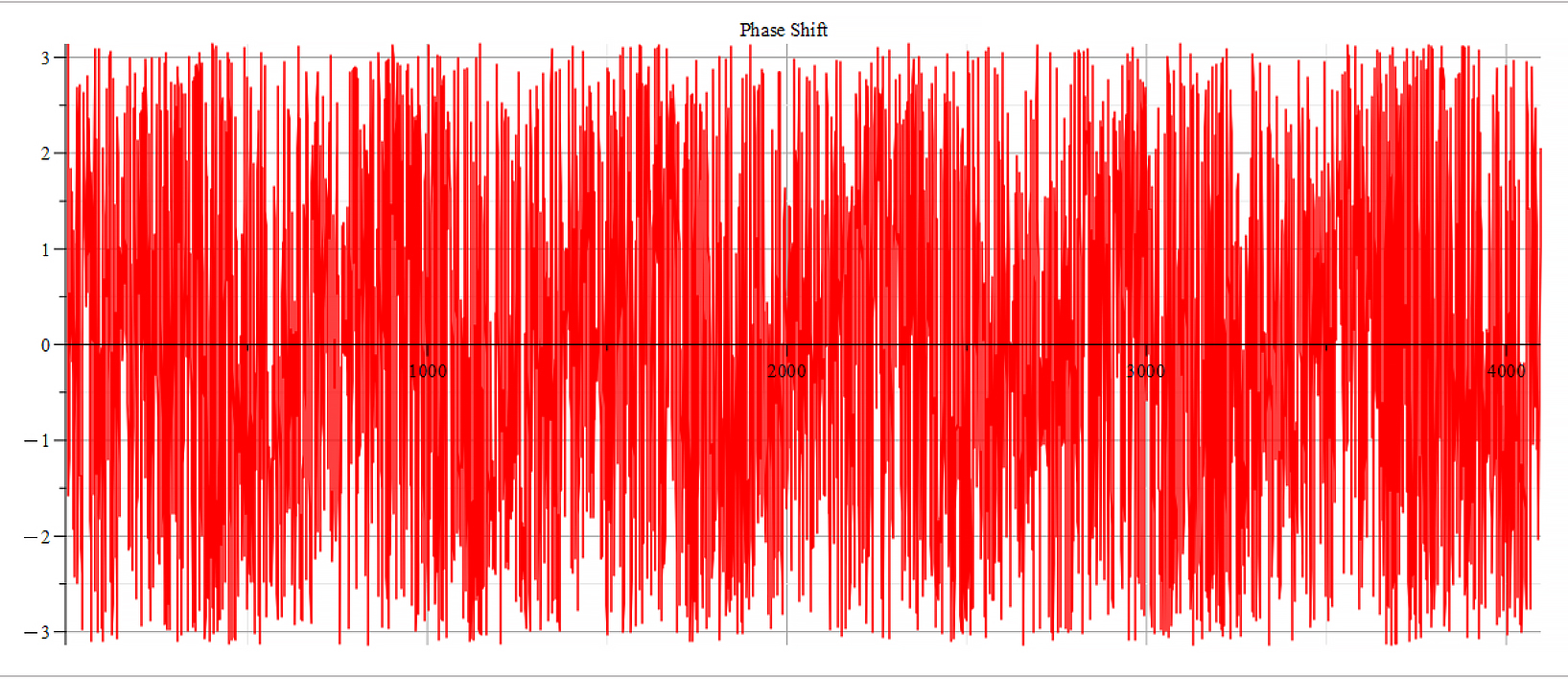
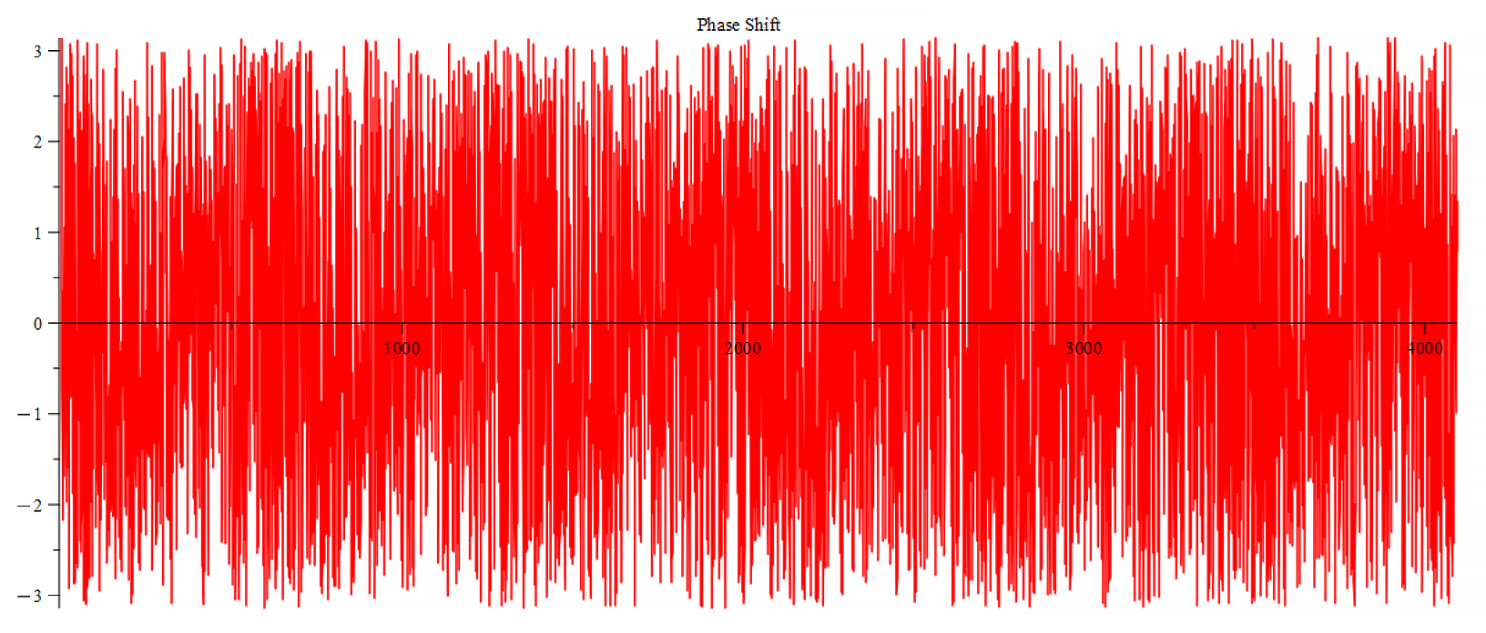
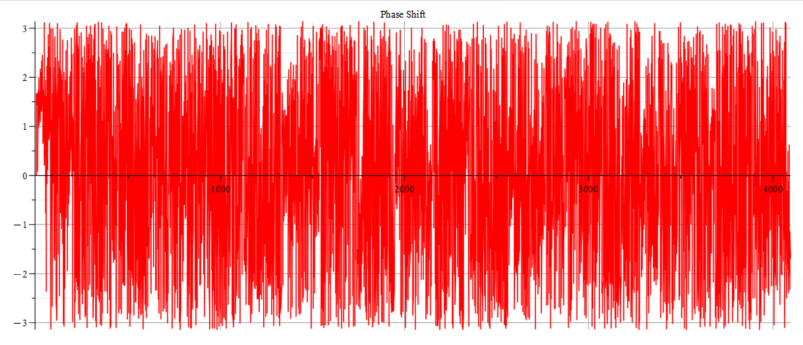
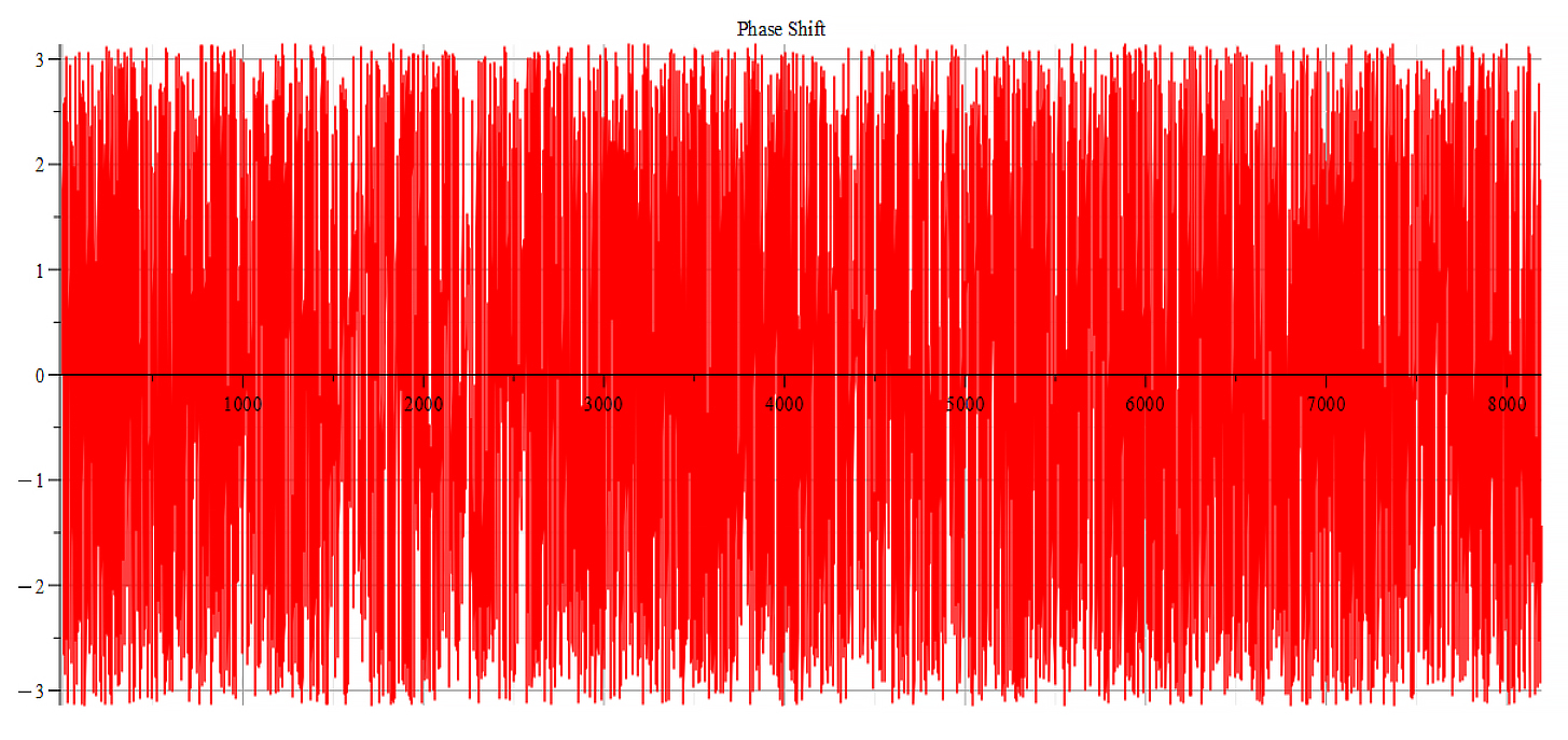
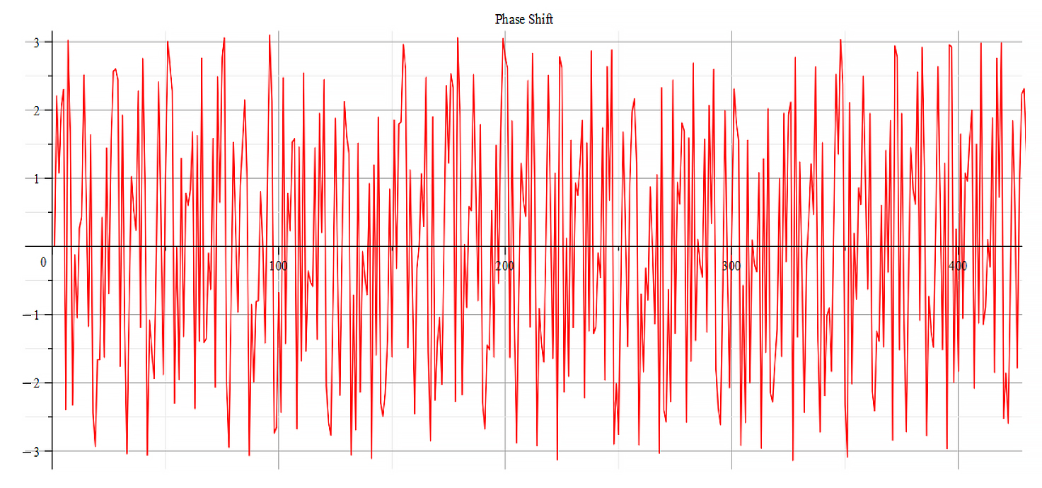
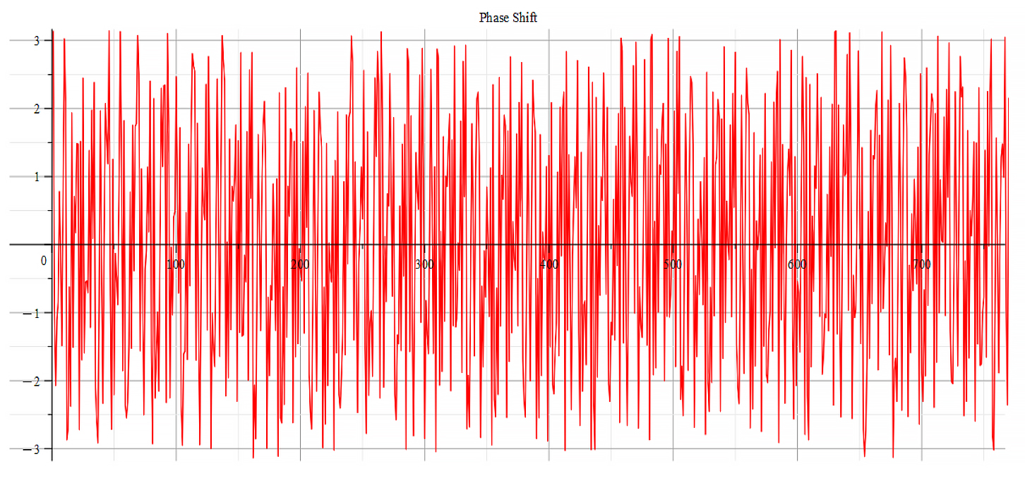
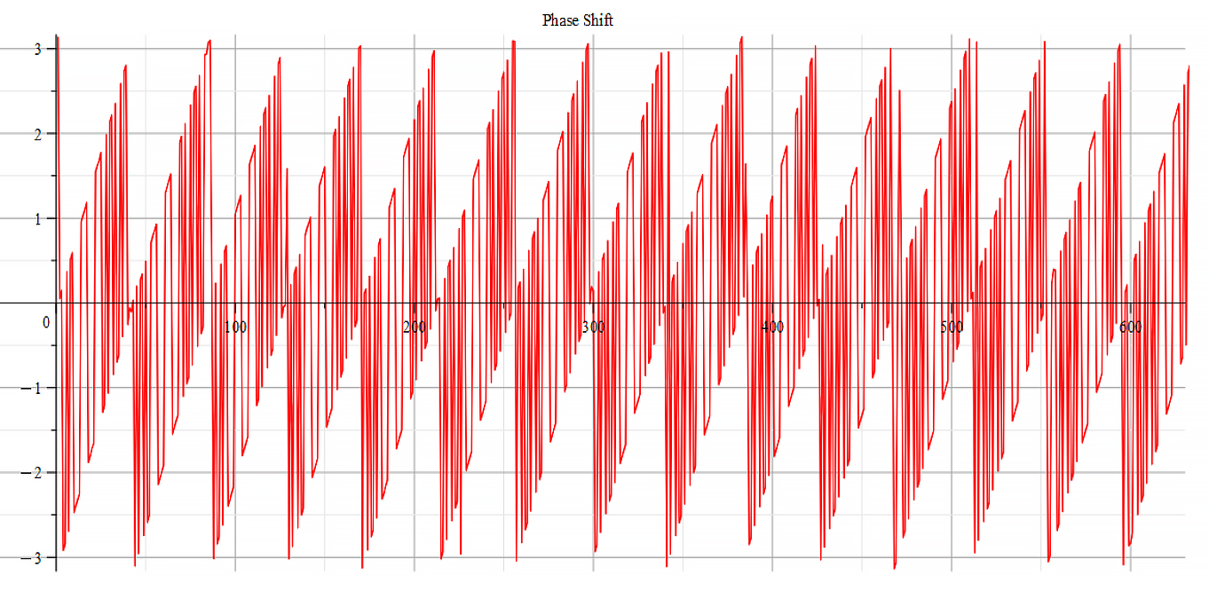
Phase shift for the following parameters: \omega={10}^{12}\ [\frac{1}{s}]; E_m={10}^{26}\ [\frac{V}{m}]; E_f={10}^{26}\ [\frac{V}{m}]
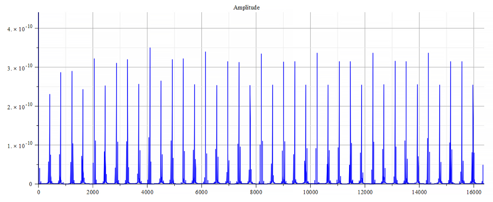
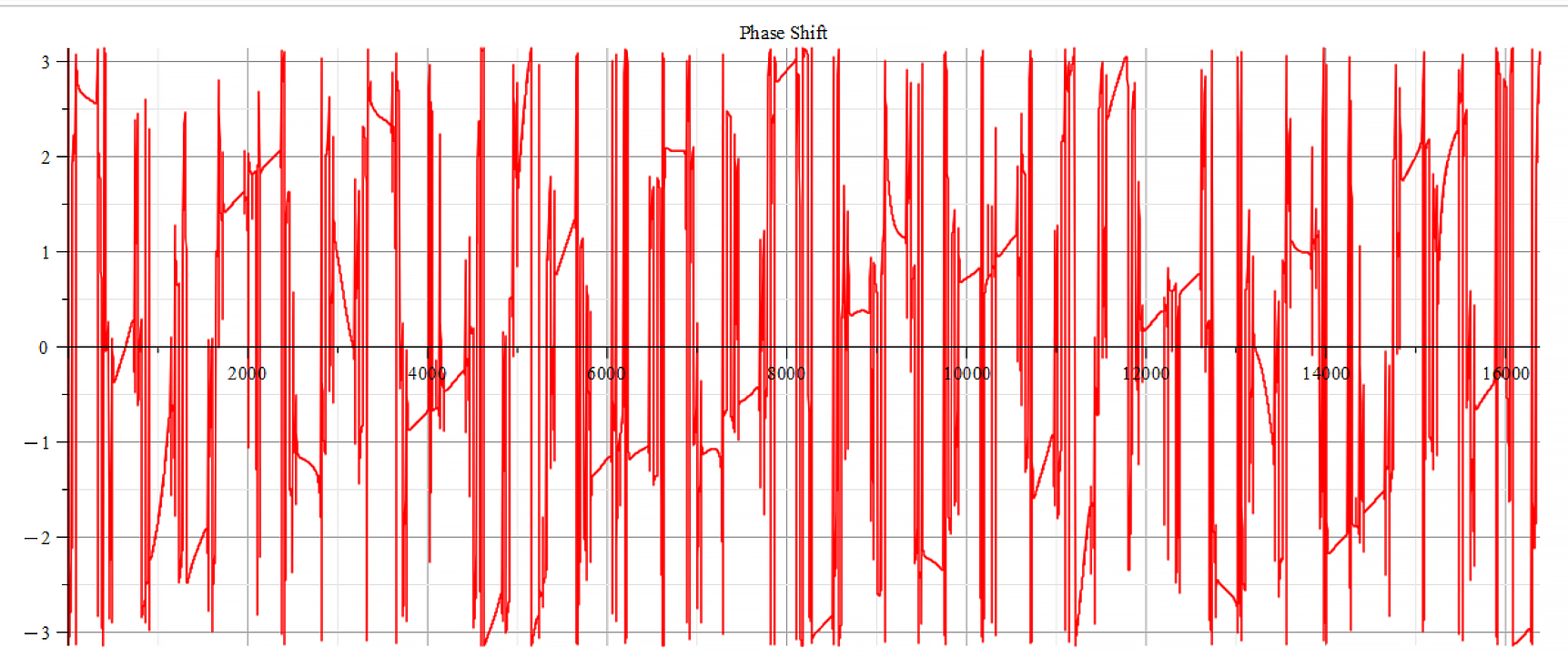
For -Ef
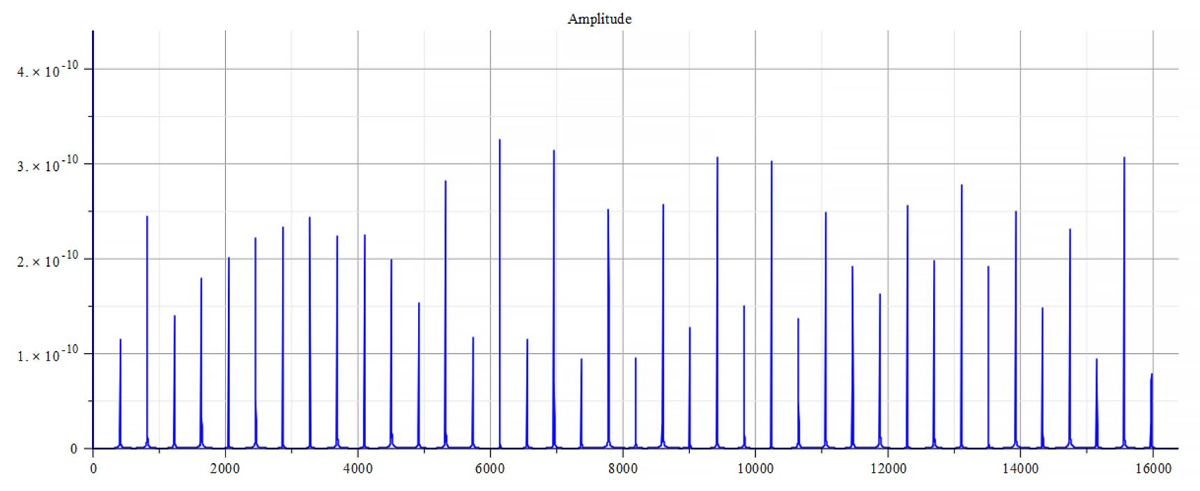
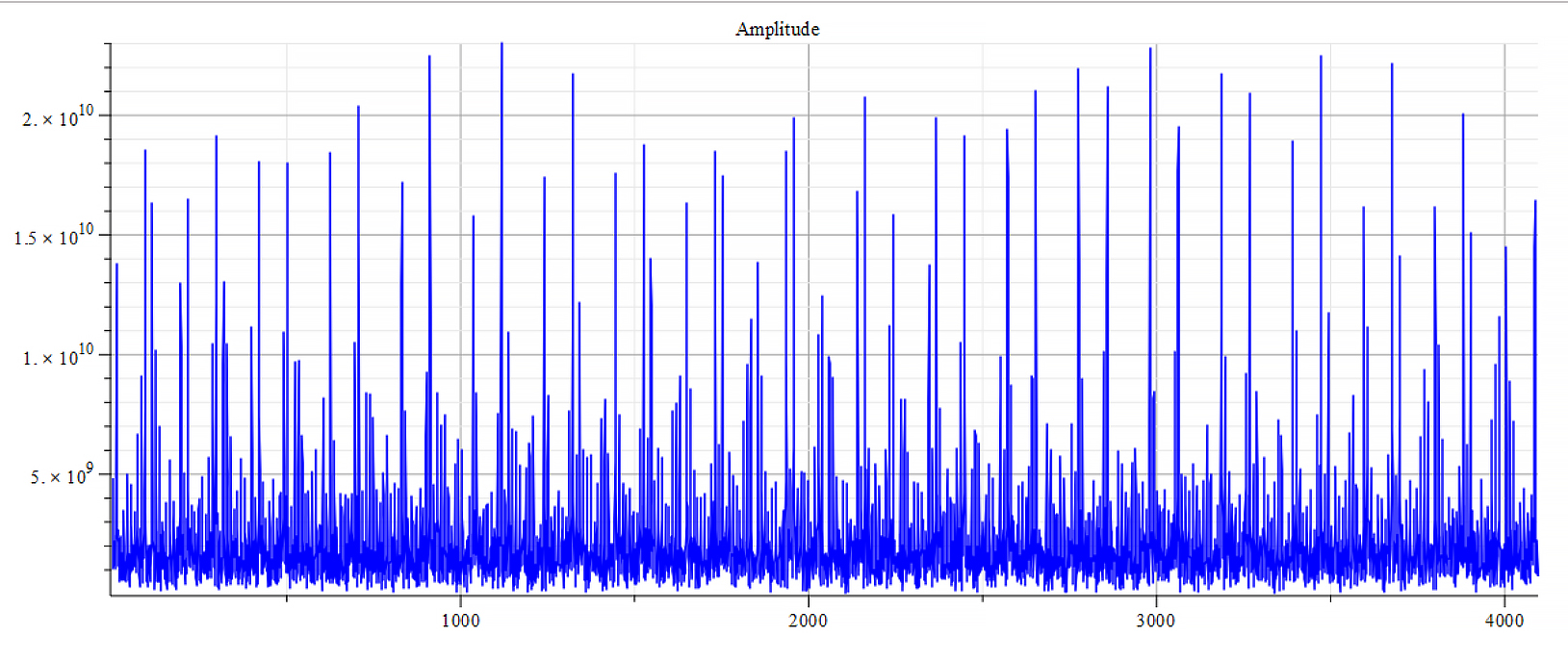
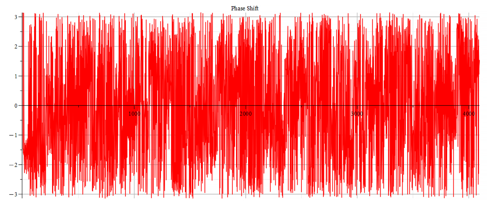
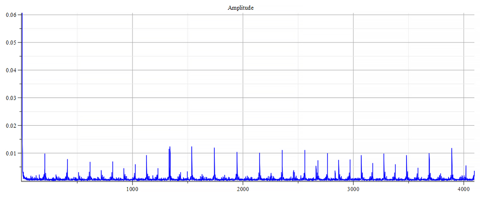
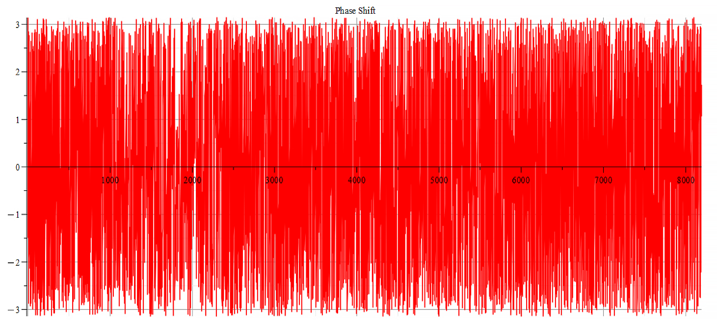
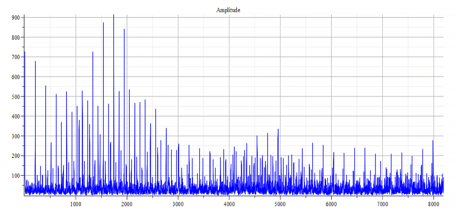
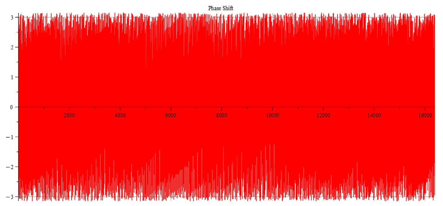
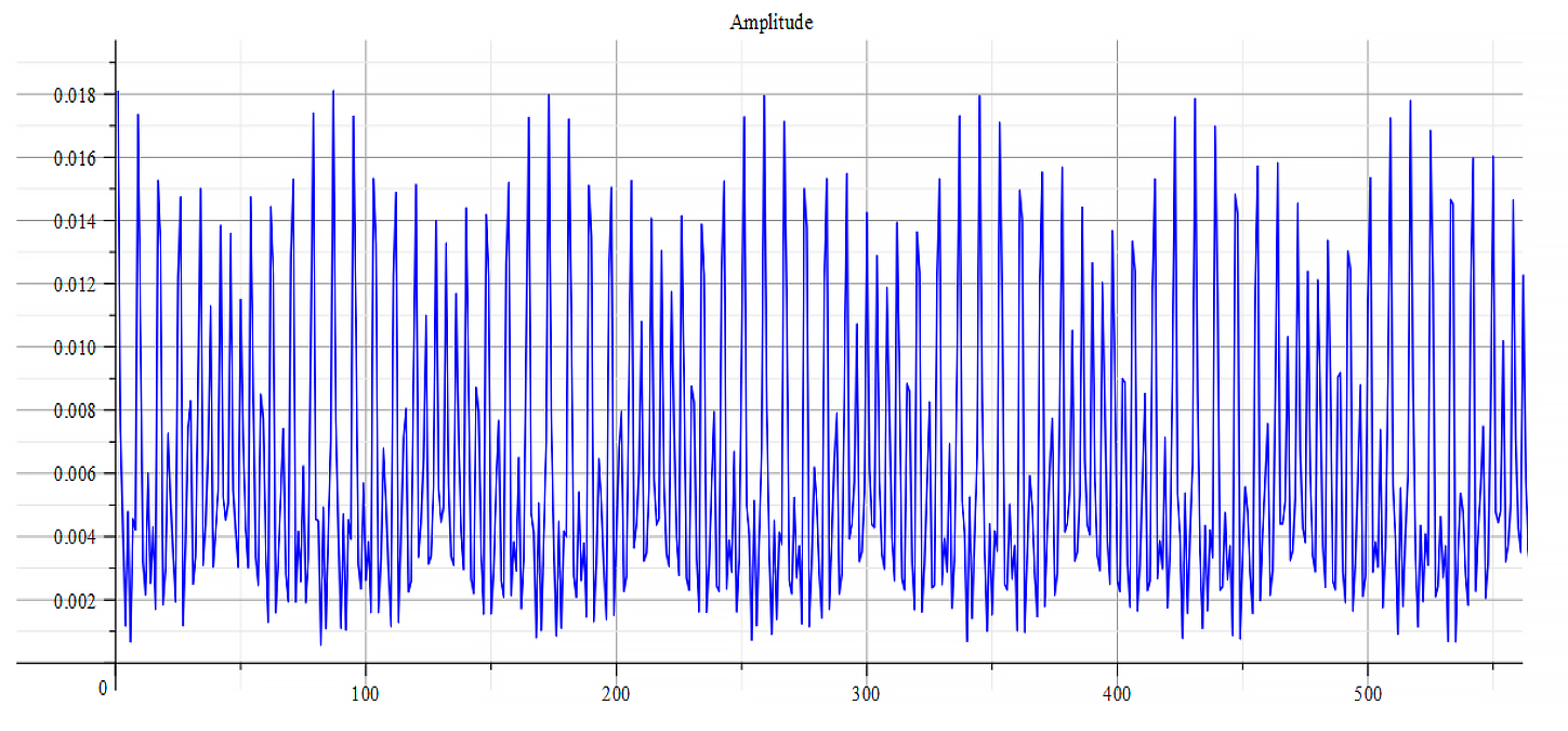
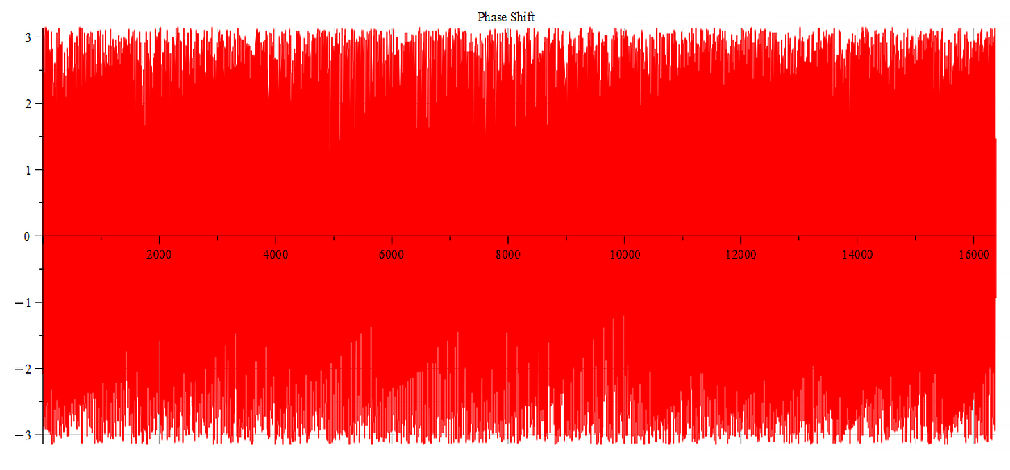
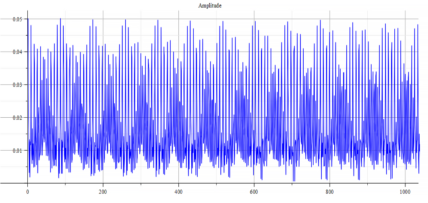
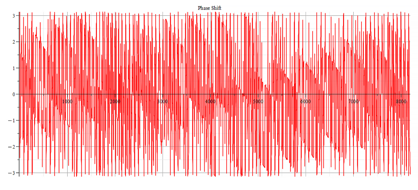
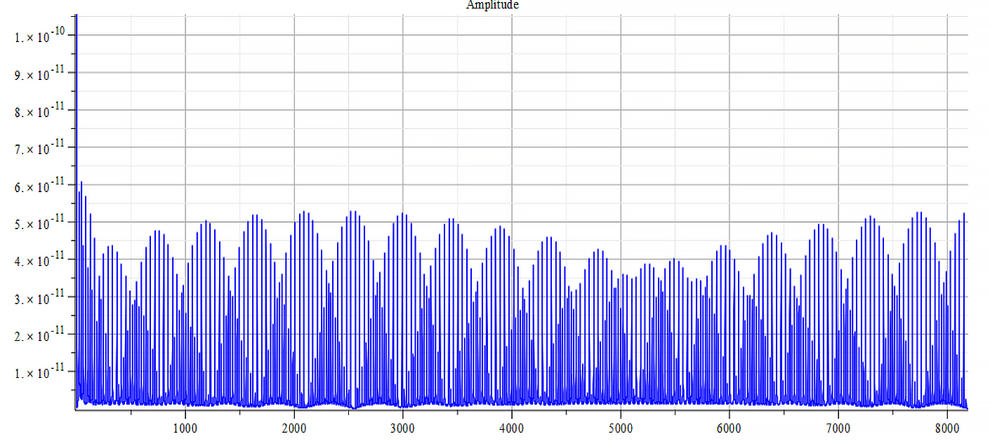
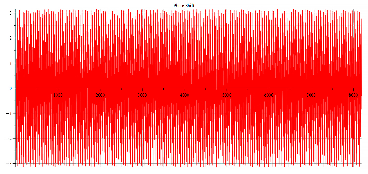
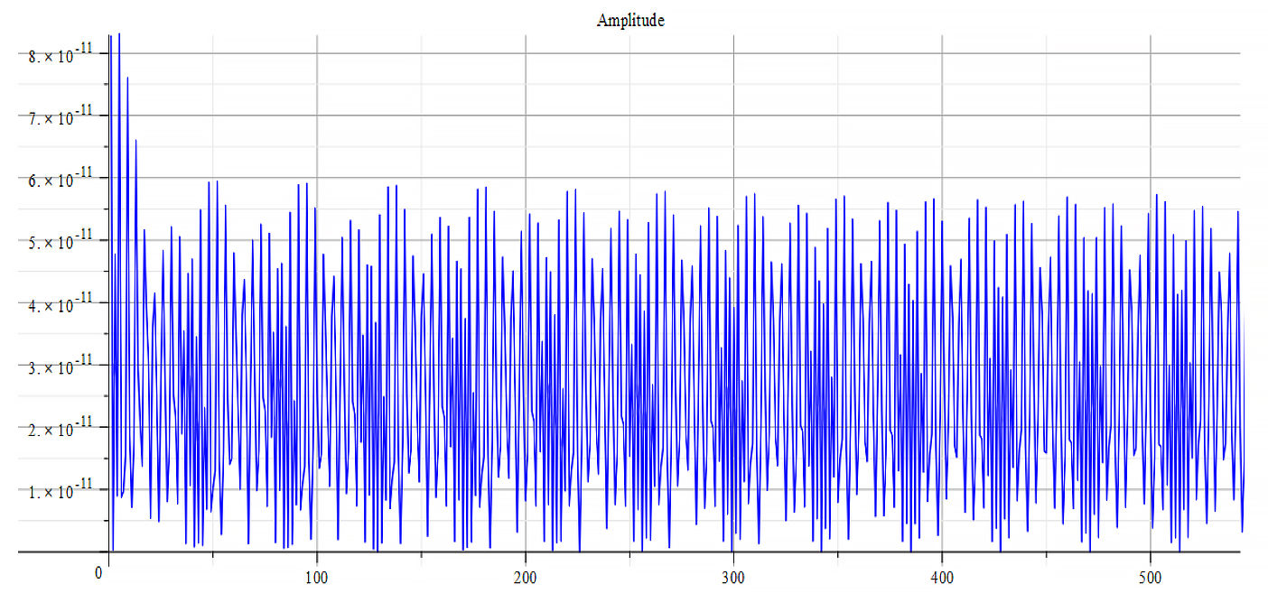
Frequency spectrum for the following parameters: \omega={10}^{12}\ [\frac{1}{s}]; E_m={10}^{26}\ [\frac{V}{m}]; E_f=-{10}^{26}\ [\frac{V}{m}]
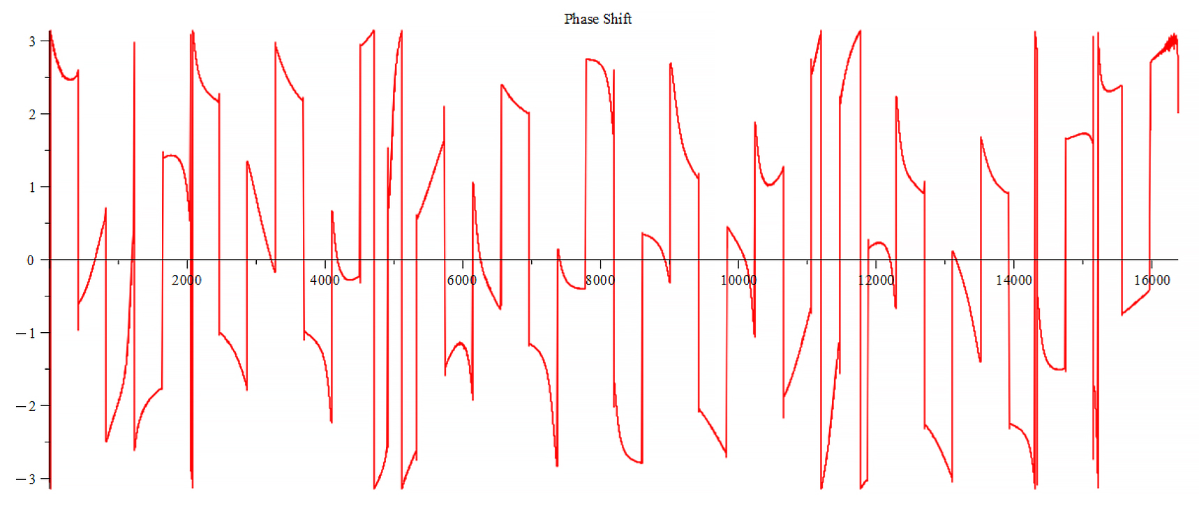
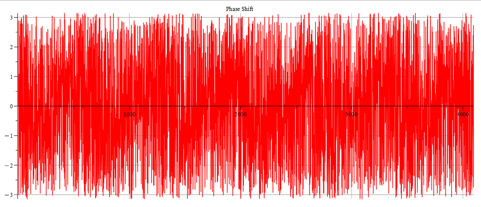
Phase shift for the following parameters: \omega={10}^{12}\ [\frac{1}{s}]; E_m={10}^{26}\ [\frac{V}{m}]; E_f=-{10}^{26}\ [\frac{V}{m}]
For +Ef
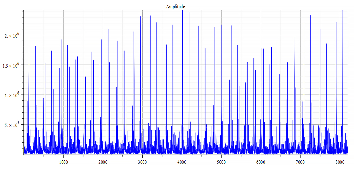
Frequency spectrum for the following parameters: \omega={10}^{14}\ [\frac{1}{s}]; E_m={10}^{26}\ [\frac{V}{m}]; E_f={2.5\ 10}^{26}\ [\frac{V}{m}]
Phase shift for the following parameters: \omega={10}^{14}\ [\frac{1}{s}]; E_m={10}^{26}\ [\frac{V}{m}]; E_f={2.5\ 10}^{26}\ [\frac{V}{m}]
For -Ef
Frequency spectrum for the following parameters: \omega={10}^{14}\ [\frac{1}{s}]; E_m={10}^{26}\ [\frac{V}{m}]; E_f=-{2.5\ 10}^{26}\ [\frac{V}{m}]
Phase shift for the following parameters: \omega={10}^{14}\ [\frac{1}{s}]; E_m={10}^{26}\ [\frac{V}{m}]; E_f=-{2.5\ 10}^{26}\ [\frac{V}{m}]
For +Ef
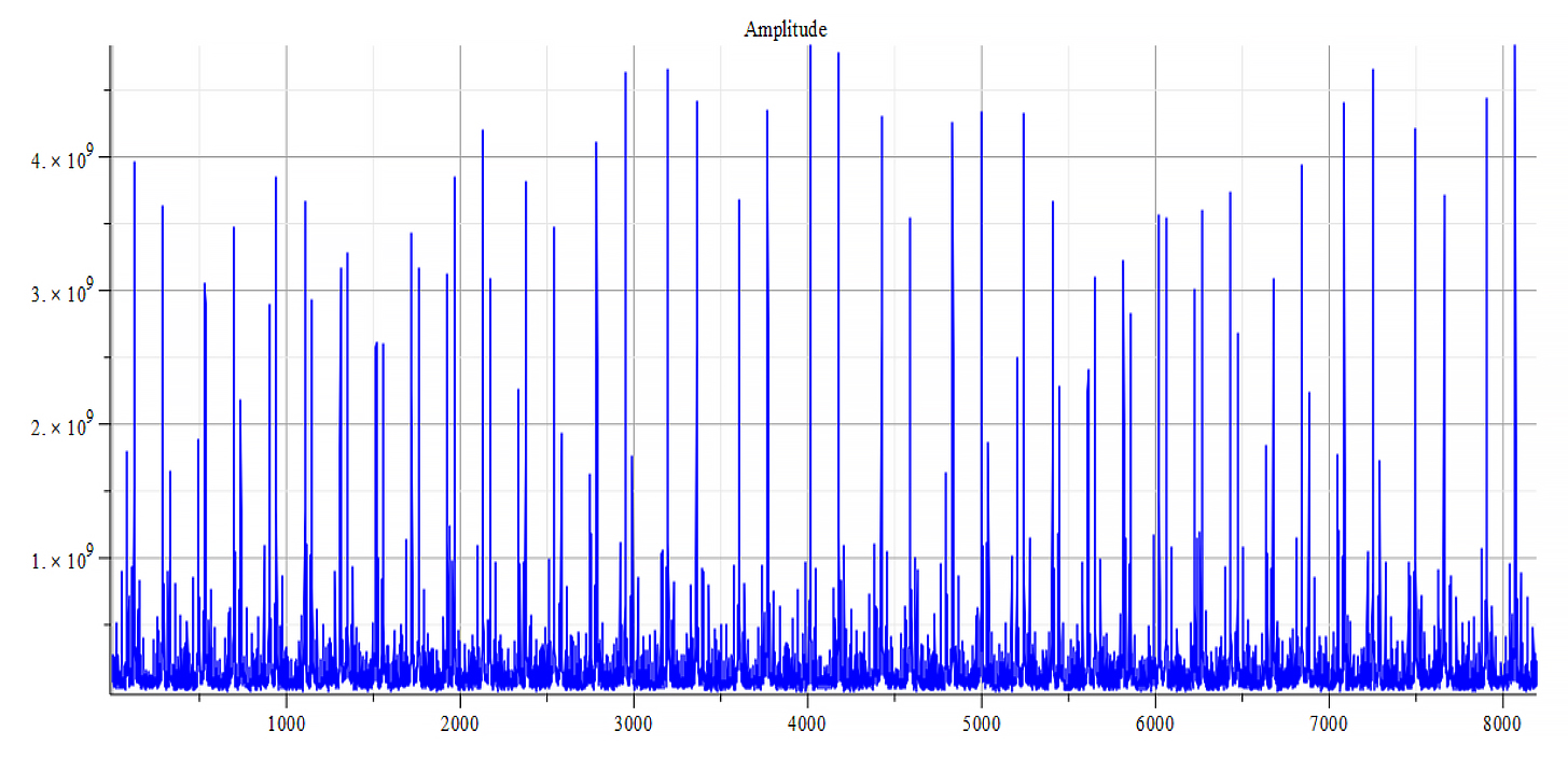
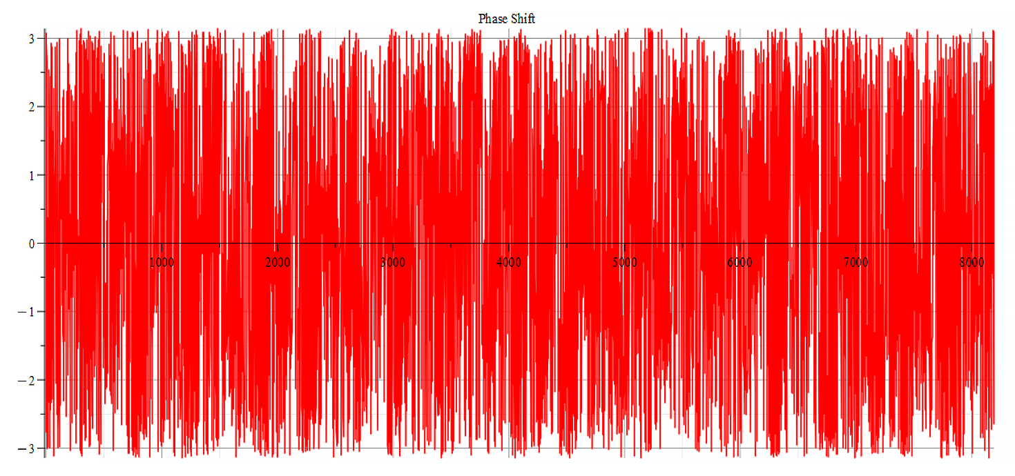
Frequency spectrum for the following parameters: \omega={10}^{17}\ [\frac{1}{s}]; E_m={10}^{26}\ [\frac{V}{m}]; E_f={2.5\ 10}^{26}\ [\frac{V}{m}]
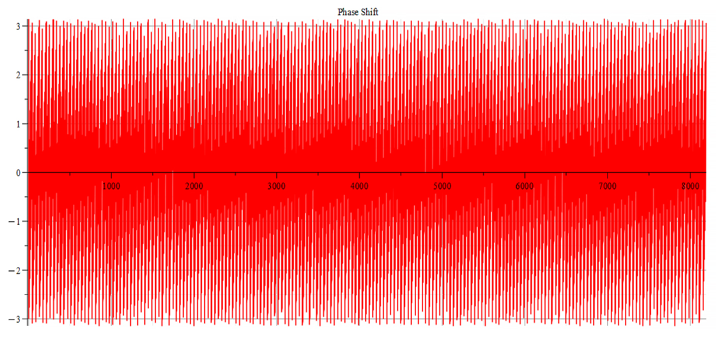
Phase shift for the following parameters: \omega={10}^{17}\ [\frac{1}{s}]; E_m={10}^{26}\ [\frac{V}{m}]; E_f={2.5\ 10}^{26}\ [\frac{V}{m}]
For -Ef
The graphs are very similar for \ +{E}_{f}. The frequency spectrum always shows the same main frequency and harmonics. However, there are some changes in amplitudes, and in the phase behavior.
From the Fourier frequency analysis, we see that the main frequency is: f_0=1.6\ {10}^{14}\ [Hz].
In general, the main frequency and harmonics are given by the following formula:
f_n=f_0+nf_0, n=0,\ 1,\ 2,\ 3…
II.b Refractive Index Analysis due to Force caused by Static Field plus Wave (4) – Partial or Total Energy Absorption
When the nucleus is under the action of external forces, and if it doesn’t break apart, then we can assume that a dynamic equilibrium state must exist. Under such circumstances, Newton’s second law requires that the sum of forces be equal to zero, {\vec{F}}{net}+{\vec{F}}{ext}=0, that is,
F_{net}=-F_{ext} (9)
Recall that the net nuclear force has already been written in terms of the index of refraction in Part-1, Eq. (23a):
{\vec{F}}{net}=-\frac{378k q^2}{r{ep}^2\left(t\right)}\left(1-\frac{1}{n^2}+\frac{v_{ep}^2\left(t\right)r_{ep}\left(t\right)a_{ep}\left(t\right)}{n^2c^2}+\frac{1}{n^4}+\frac{2r_{ep}\left(t\right)a_{ep}\left(t\right)}{c^2}\right)\hat{r}+\frac{2279.035793k q^2\hat{r}}{r_n^2}
Now we can equate the forces according to Eq. (9), then solve for “n”,
-\frac{{3.410}^{12}\cdot q^2\left(1-\frac{1}{n^2}+\frac{r_{ep}\left(t\right)a_{ep}\left(t\right)}{n^2c^2}+\frac{1}{n^4}+\frac{2r_{ep}\left(t\right)a_{ep}\left(t\right)}{c^2}\right)}{r_{ep}^2\left(t\right)}+\frac{{2.0510}^{13}\cdot q^2}{r_n^2}=-\frac{2\pi\varepsilon_0v_w}{3c K^3r_n}\cdot\left(-\frac{3E_m^2\sin{\left(2Kr_n-2\omega t\right)}}{8}-12E_fE_m\sin{\left(Kr_n-\omega t\right)}+\frac{3E_m^2\left(K^2r_n^2-\frac{1}{2}\right)\sin{\left(2\omega t\right)}}{4}+\frac{3E_m^2r_nK\cos{\left(2\omega t\right)}}{4}+6E_fE_m\left(K^2r_n^2-2\right)\sin{\left(\omega t\right)}+r_n\left(12E_fE_m\cos{\left(\omega t\right)}+K^2r_n^2\left(E_f^2+\frac{E_m^2}{2}\right)\right)K\right) (10)
The refractive index “n” is a somewhat long-expression which is nonsense to copy here. Some plots as examples are shown below, where the main used parameters are:
r_n=3.5\ {10}^{-15}\ [m]; A_e=2\ {10}^{-16}\ [m]; A_p={10}^{-3}A_e\ [m]; N_0=378; N_s=312
\omega_e={10}^{15}\ [\frac{1}{s}]; \omega_p={10}^{16}\ [\frac{1}{s}]
While for the wave: v_w=v_{ep}\left(t\right); K=\frac{\omega}{v_{ep}\left(t\right)}
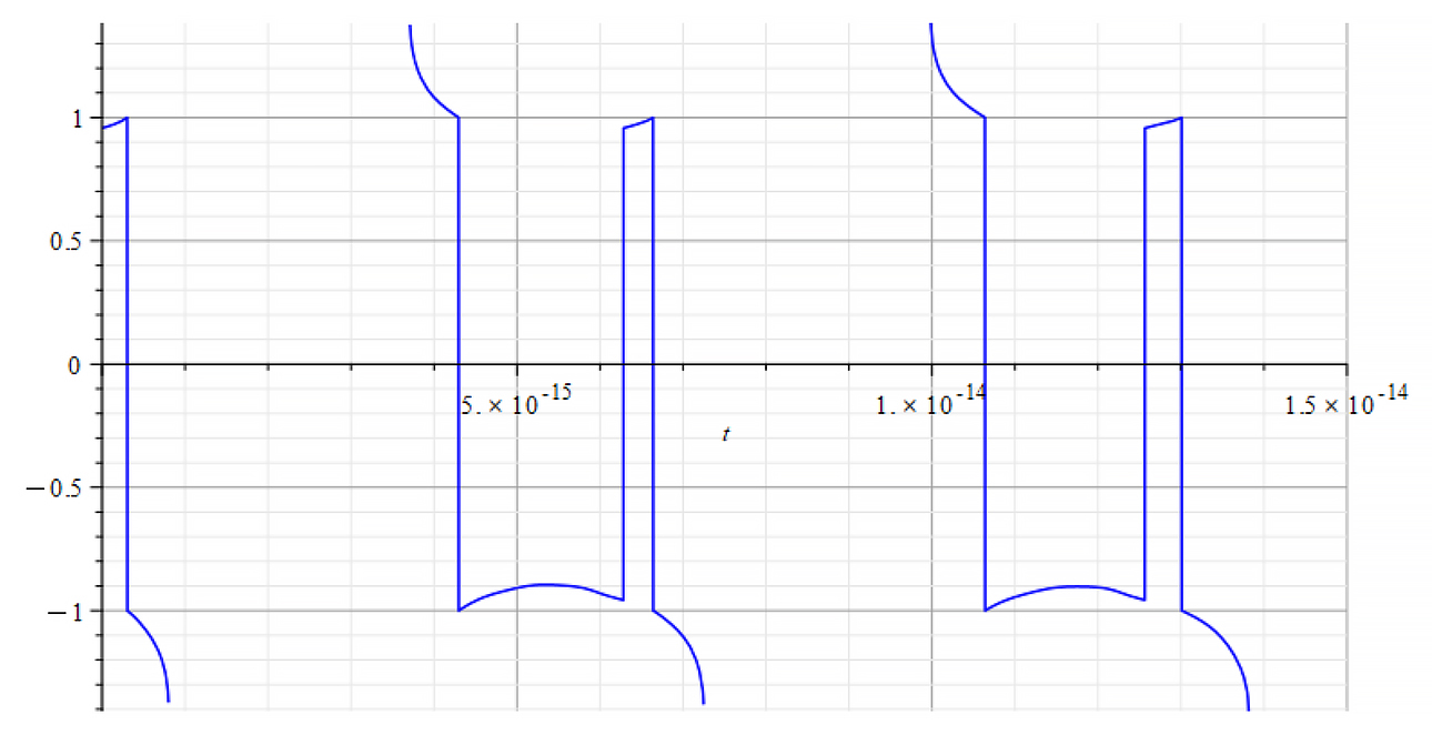
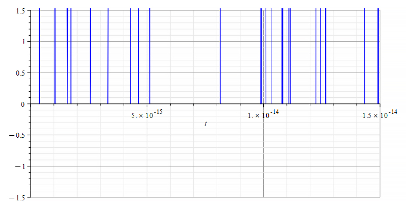
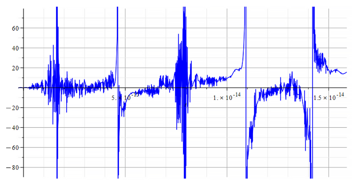
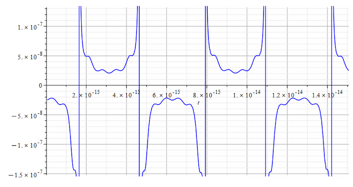
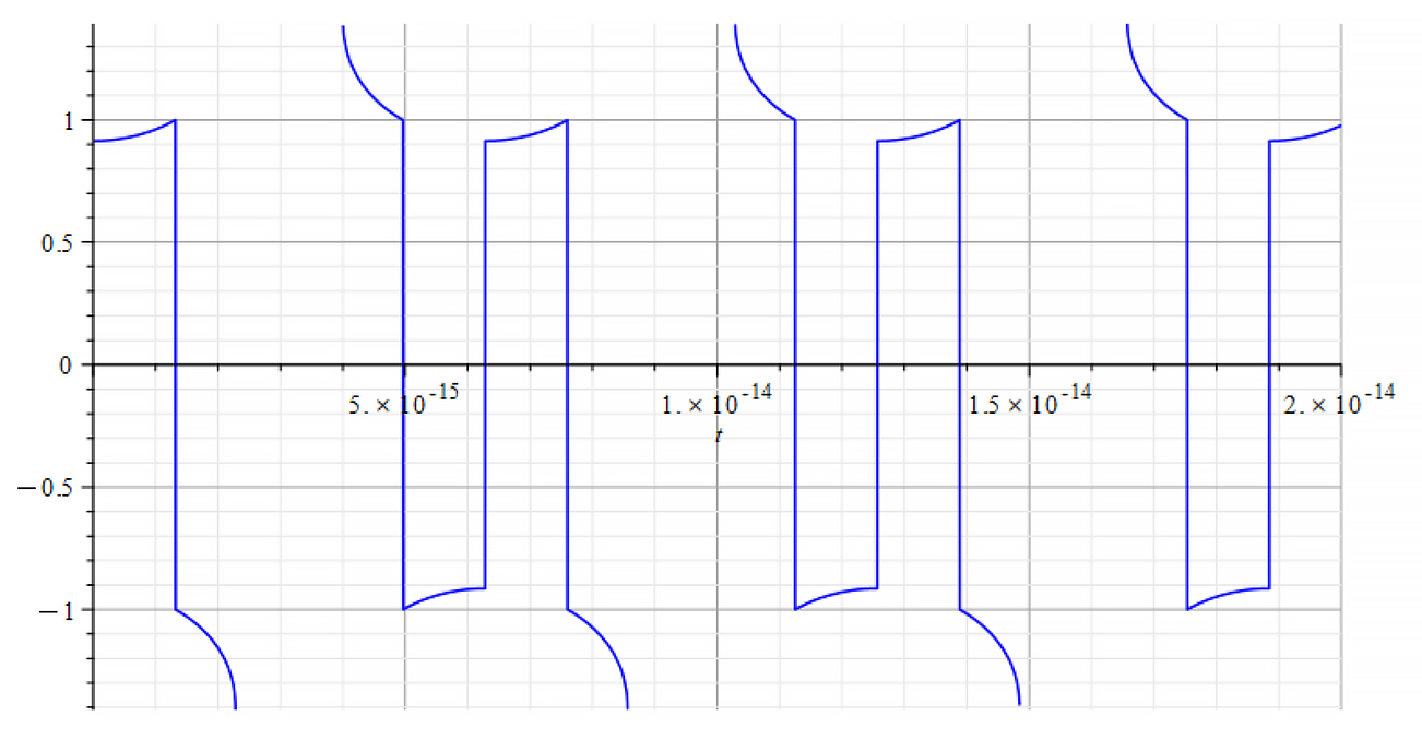
 |  |
| +{E}_{f} Refractive Index vs. time for the following parameters: \omega={10}^{12}\ [\frac{1}{s}]; E_m={10}^{26}\ [\frac{V}{m}]; E_f={10}^{26}\ [\frac{V}{m}] | -{E}_{f} Refractive Index vs. time for the following parameters: \omega={10}^{12}\ [\frac{1}{s}]; E_m={10}^{26}\ [\frac{V}{m}]; E_f={-10}^{26}\ [\frac{V}{m}] |
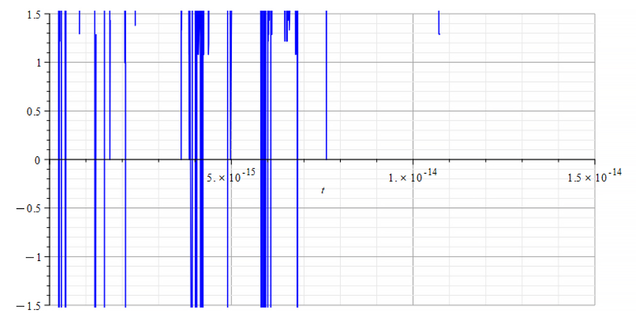
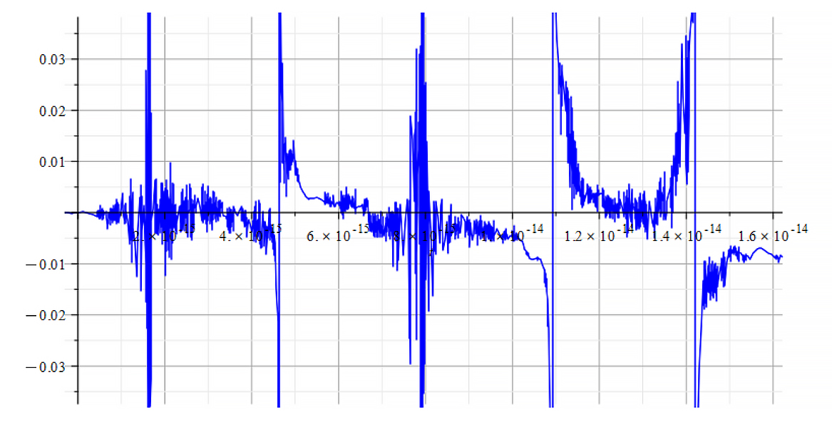
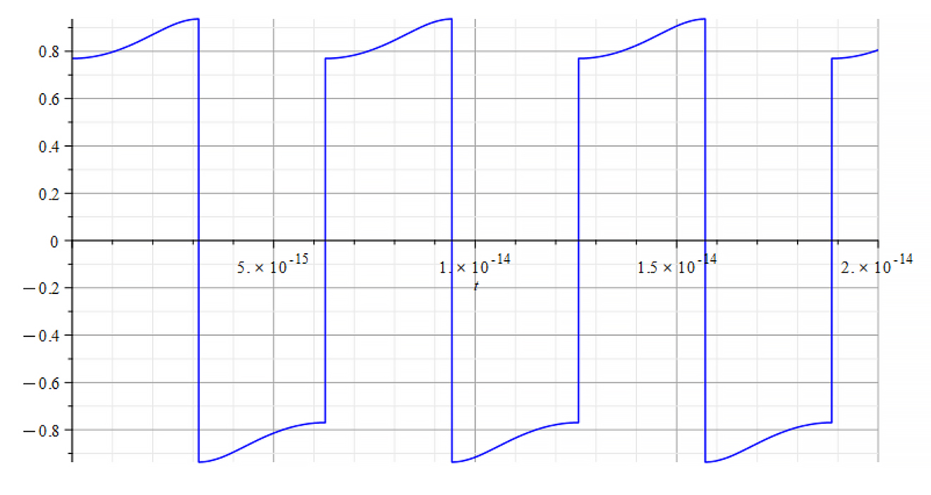
 | 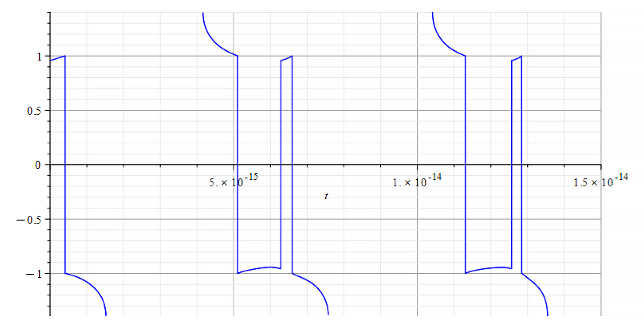 |
| +{E}_{f} Refractive Index vs. time for the following parameters: \omega={10}^{14}\ [\frac{1}{s}]; E_m={10}^{26}\ [\frac{V}{m}]; E_f={2.5\ 10}^{26}\ [\frac{V}{m}] | -{E}_{f} Refractive Index vs. time for the following parameters: \omega={10}^{14}\ [\frac{1}{s}]; E_m={10}^{26}\ [\frac{V}{m}]; E_f={-2.5\ 10}^{26}\ [\frac{V}{m}] |
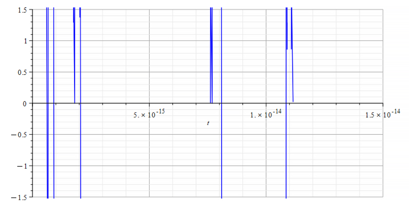
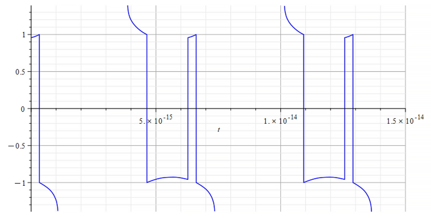 | |
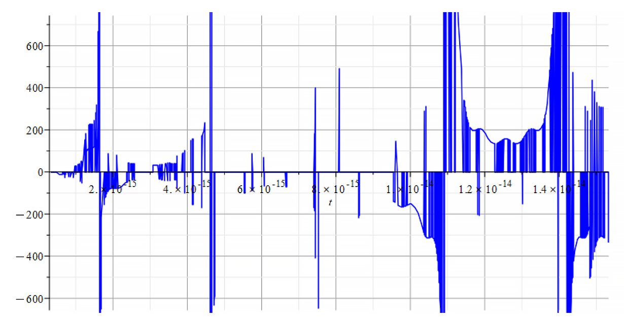
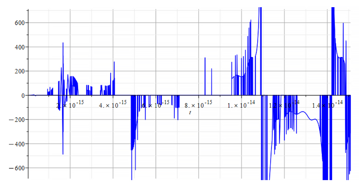
| +{E}_{f} Refractive Index vs. time for the following parameters: \omega={10}^{17}\ [\frac{1}{s}]; E_m={10}^{26}\ [\frac{V}{m}]; E_f={\pm2.5\ 10}^{26}\ [\frac{V}{m}] | -{E}_{f} Same result for both polarities |
II.c Comparison of Mass with Refractive Index Behavior due to Force caused by Static Field plus Wave (4) – Partial or Total Energy Absorption
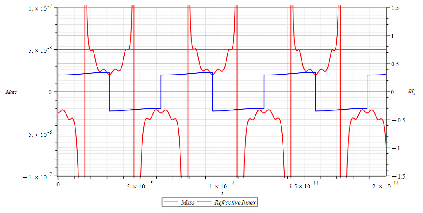
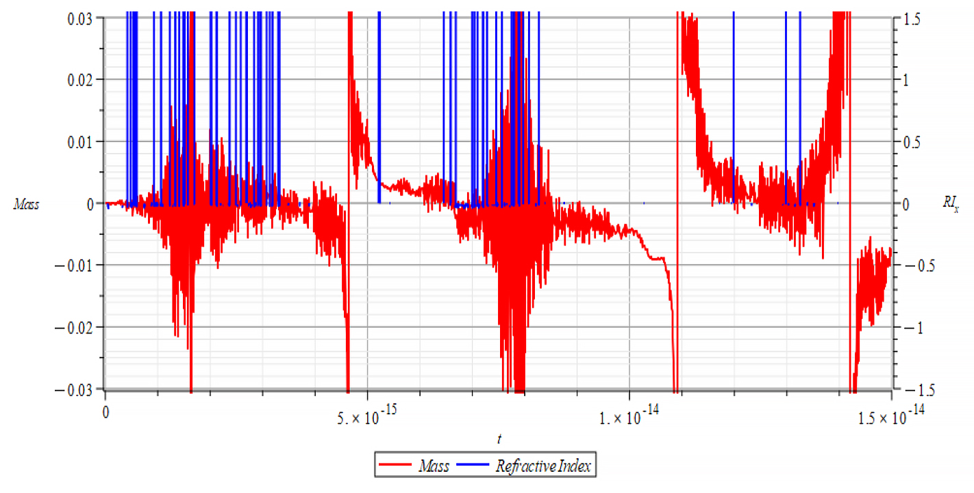
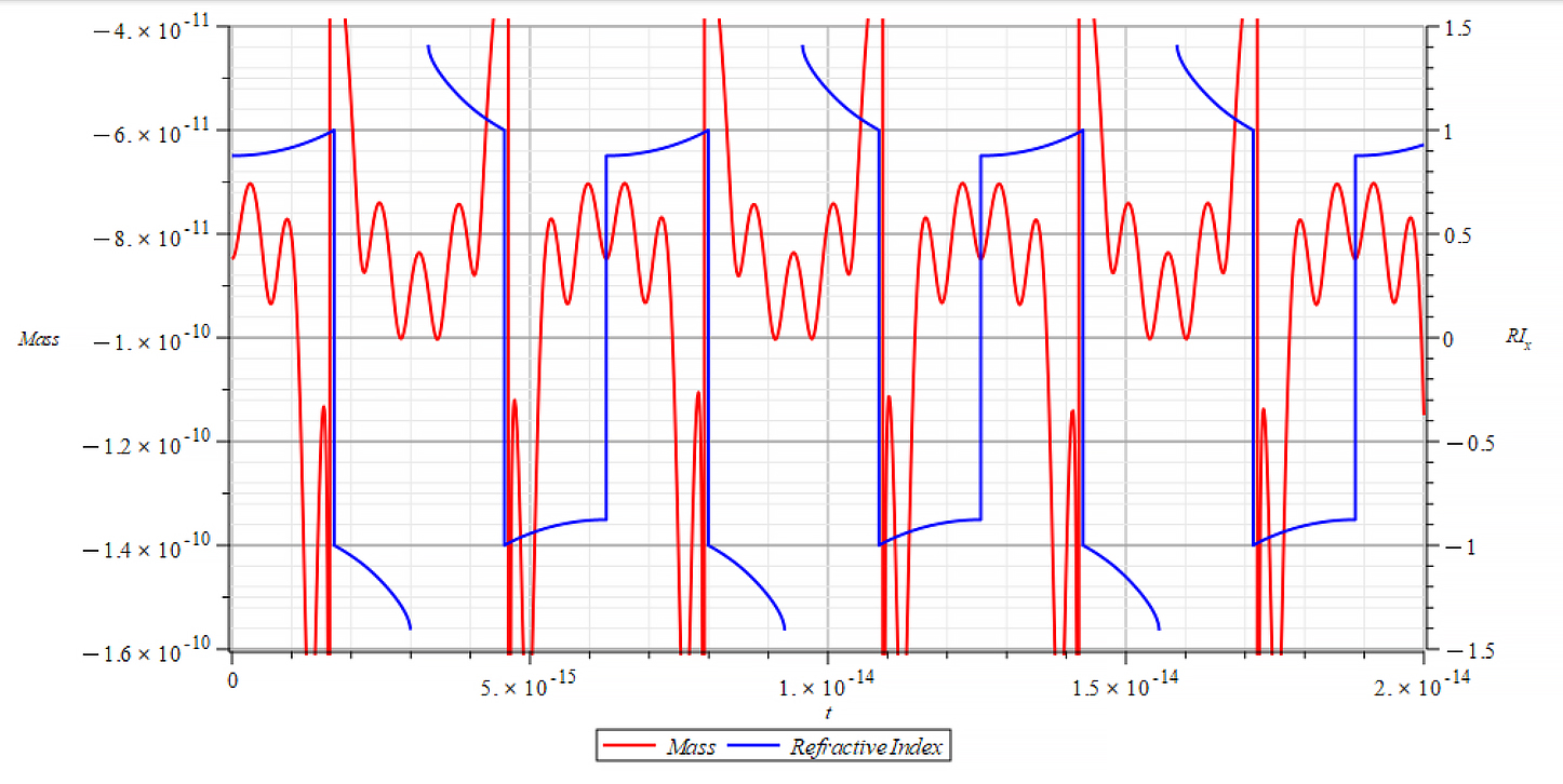
To analyze the changes in the refractive index “n” with respect to changes in nuclear mass, overlaid graphs of both quantities are shown below, which uncover interesting results.
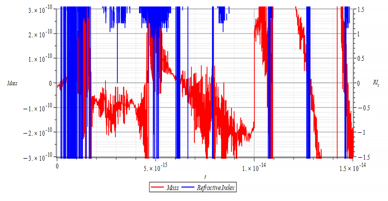
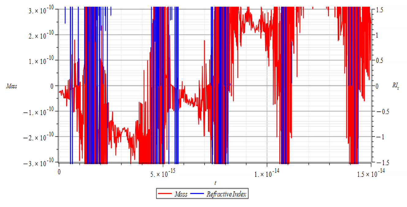
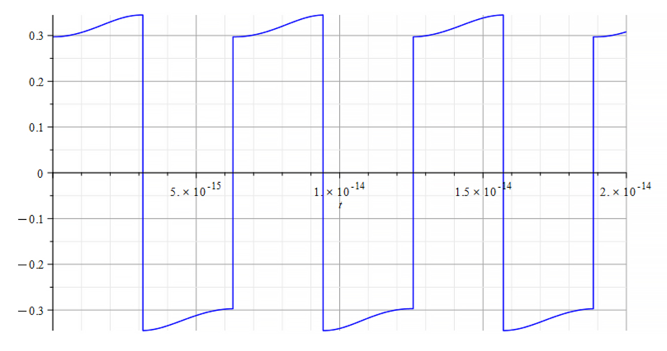
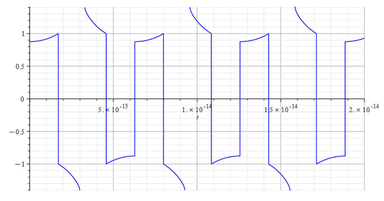
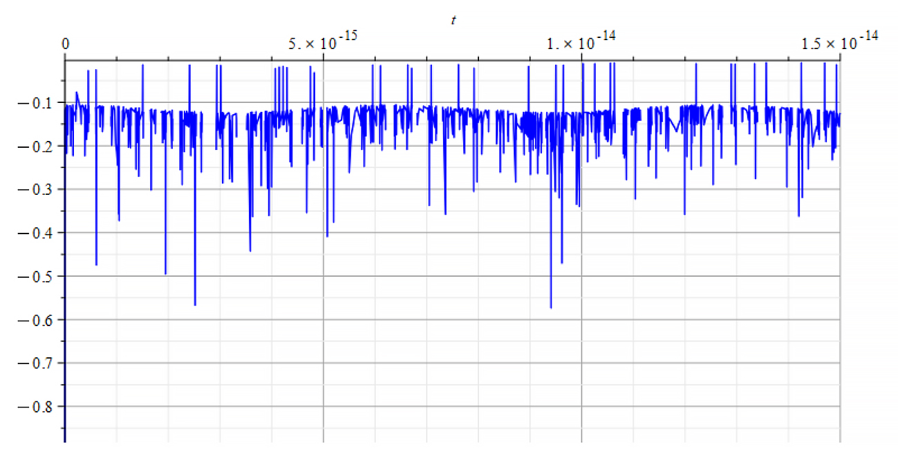
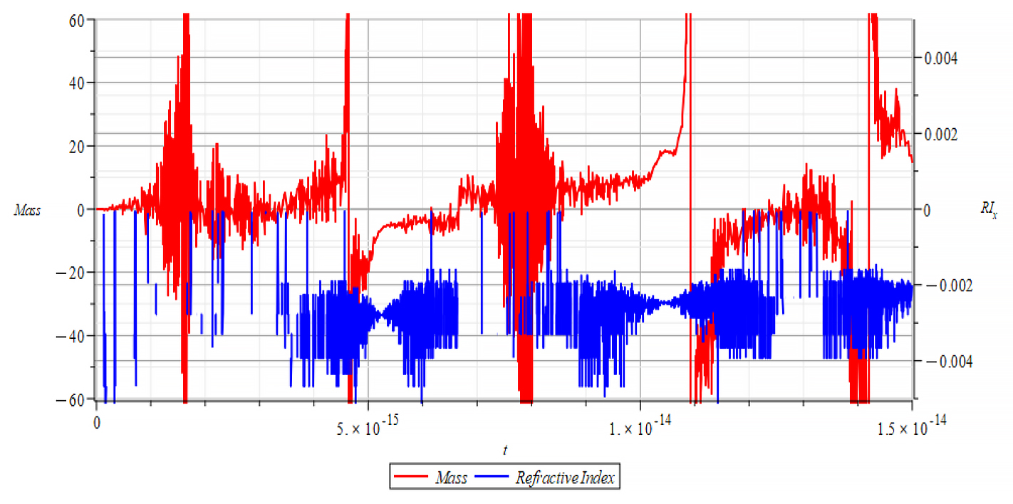
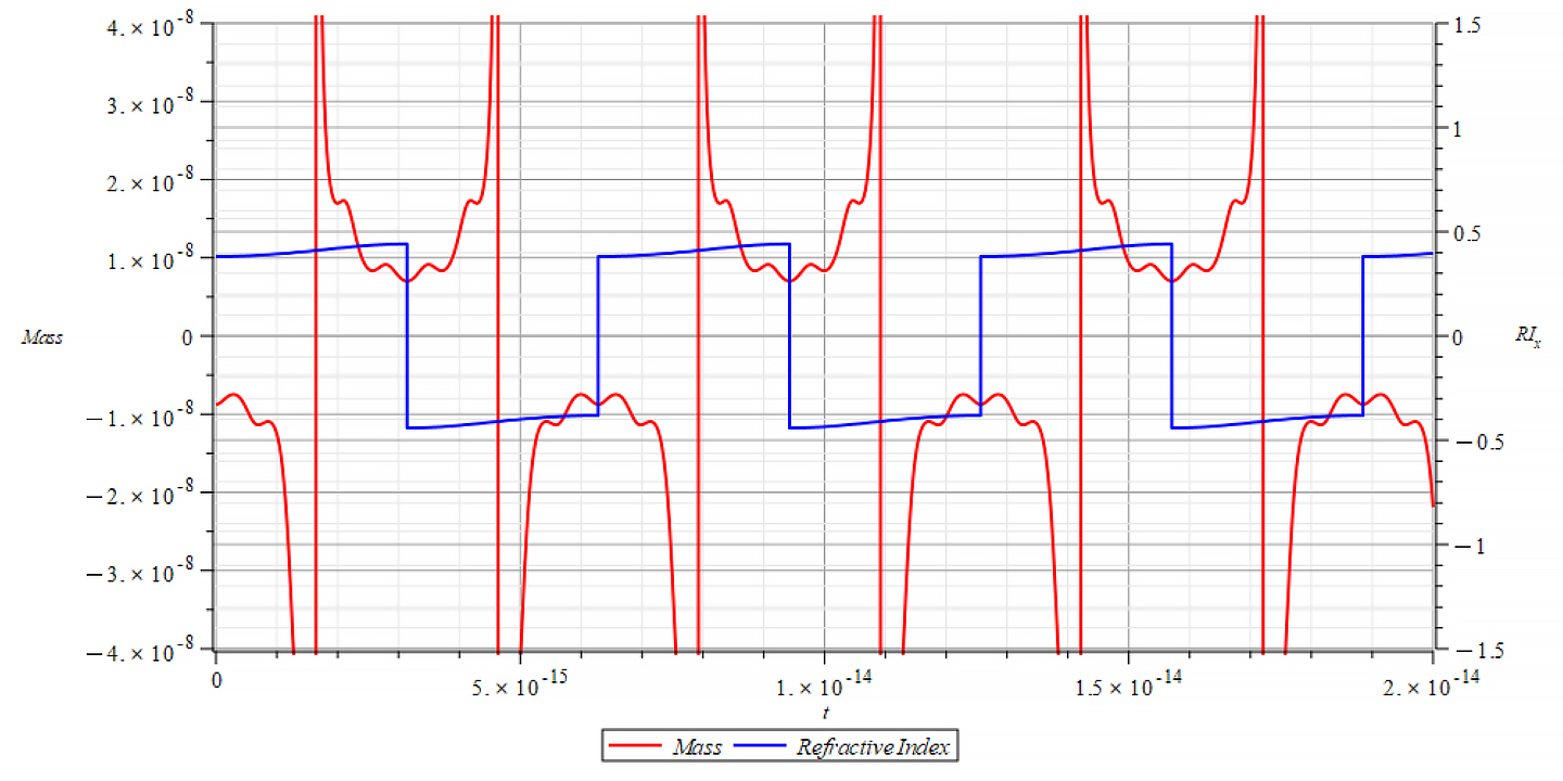
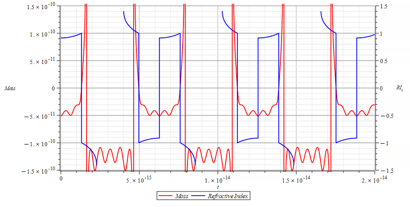
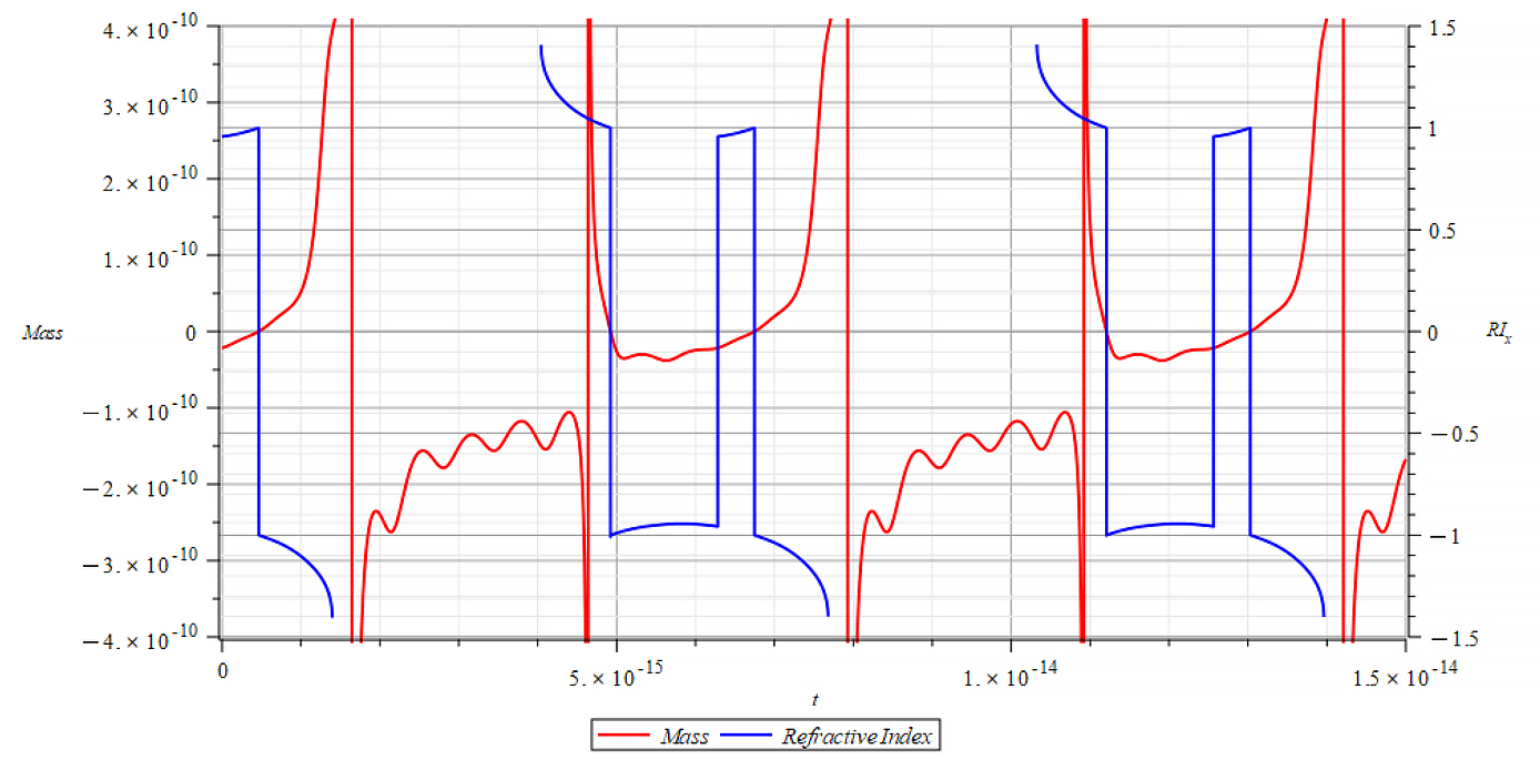 |  |
| +{E}_{f} Mass & Refractive Index vs. time for the following parameters: \omega={10}^{12}\ [\frac{1}{s}]; E_m={10}^{26}\ [\frac{V}{m}]; E_f={10}^{26}\ [\frac{V}{m}] | -{E}_{f} Mass & Refractive Index vs. time for the following parameters: \omega={10}^{12}\ [\frac{1}{s}]; E_m={10}^{26}\ [\frac{V}{m}]; E_f={-10}^{26}\ [\frac{V}{m}] |
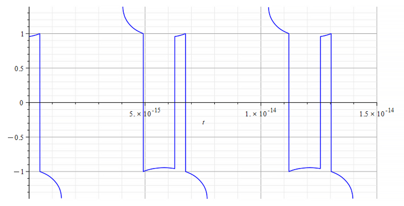
The Refractive Index oscillates, and the period switches between n=±1 at the crossing point of m=0, as well at some point with mass plot slope =0. It seems that the refractive index depends on the derivative of the mass, by changing the sign at both m=0 points, that is,
n\ \propto\pm\frac{dm}{dt}
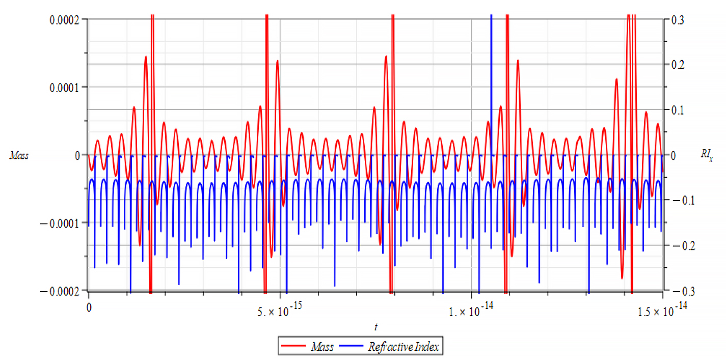
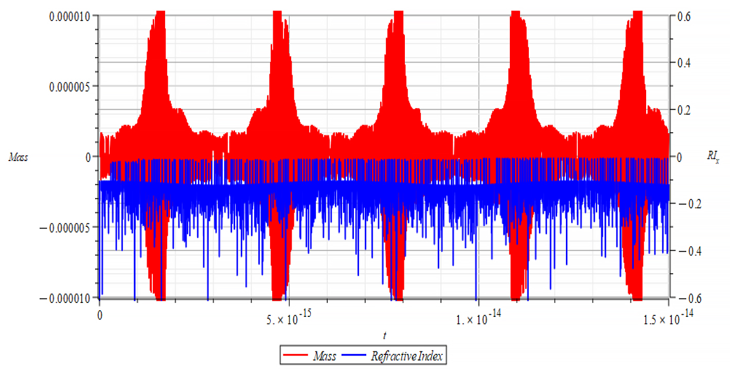
 |  |
| +{E}_{f} Mass & Refractive Index vs. time for the following parameters: \omega={10}^{14}\ [\frac{1}{s}]; E_m={10}^{26}\ [\frac{V}{m}]; E_f={2.5\ 10}^{26}\ [\frac{V}{m}] | -{E}_{f} Mass & Refractive Index vs. time for the following parameters: \omega={10}^{14}\ [\frac{1}{s}]; E_m={10}^{26}\ [\frac{V}{m}]; E_f={-2.5\ 10}^{26}\ [\frac{V}{m}] |
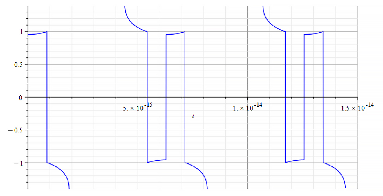
The Refractive Index oscillates, and the period switches between n=±1 at the crossing point of m=0. It seems that the refractive index depends on the derivative of the mass, by changing the sign at both m=0 points.
n\ \propto\pm\frac{dm}{dt}
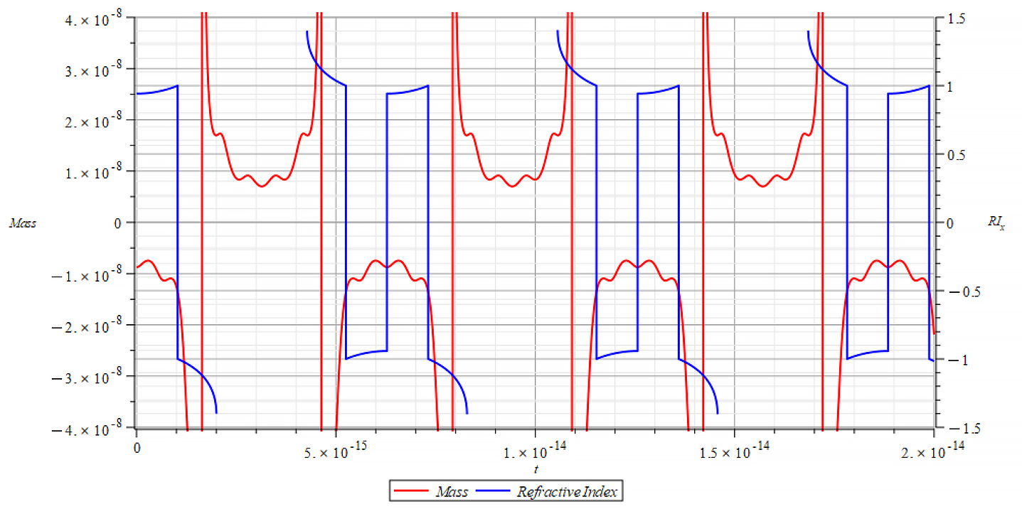
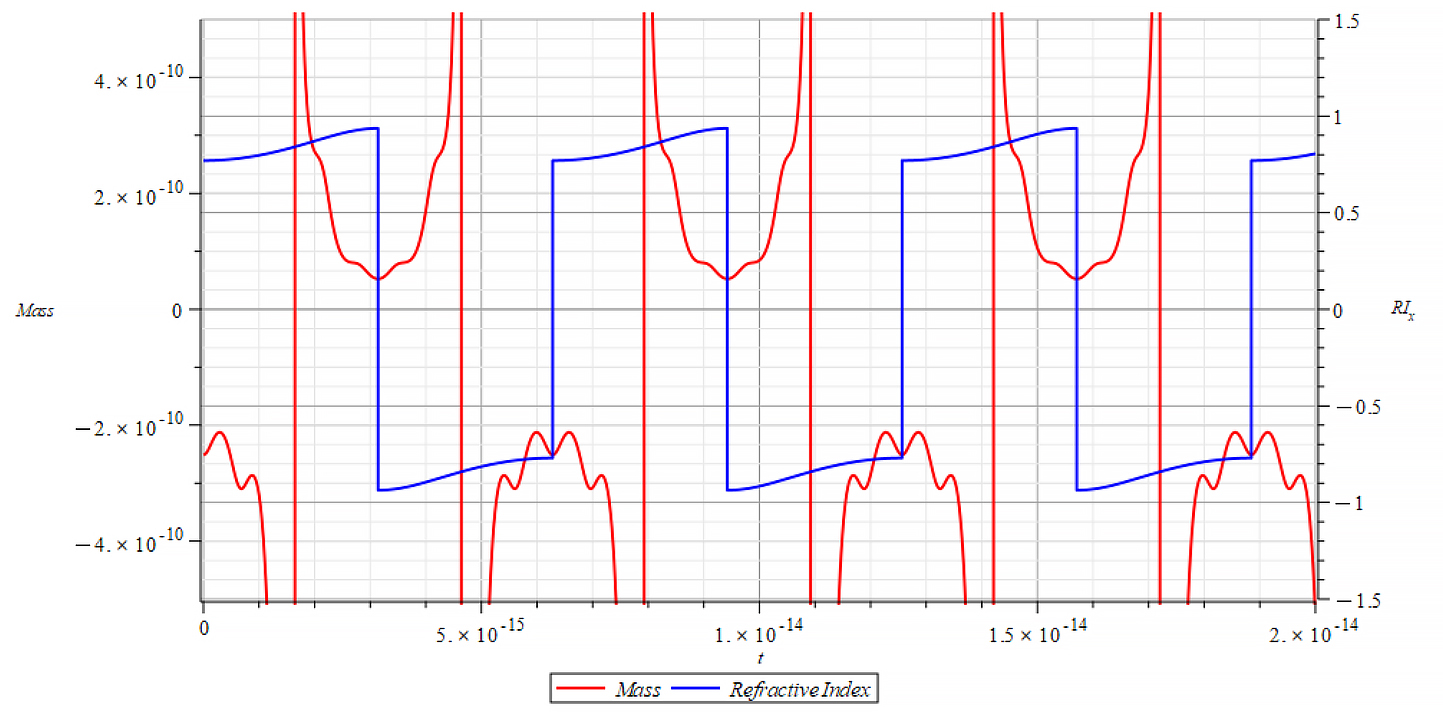
 | |
| +{E}_{f} Mass & Refractive Index vs. time for the following parameters: \omega={10}^{17}\ [\frac{1}{s}]; E_m={10}^{26}\ [\frac{V}{m}]; E_f={\pm2.5\ 10}^{26}\ [\frac{V}{m}] | -{E}_{f} Same result for both polarities |
The Refractive Index oscillates, and the period switches between n=±1 at the crossing point of m=0, as well at some point with mass plot slope =0. It seems that the refractive index depends on the derivative of the mass, by changing the sign at both m=0 points.
n\ \propto\pm\frac{dm}{dt}
This is an important result that tells us that the refractive index behavior is like a “beacon”, signaling the zones of the negative mass regime.
III.a Nuclear Mass Analysis due to Force caused by Static Field plus Wave (5) – Total Energy Transmission
The intrinsic net force in the nucleus was already defined with Eq. (23) in Part-1. Now we have the action of an external force acting on the nucleus that will interact with the internal force. By applying Newton’s second law, we have
\sum F=m_n\cdot a_{ep}=F_{net}+F_{ext} => m_n\cdot a_{ep}=F_{net}+F_{ext}
m_n=\frac{1}{a_{ep}}\cdot\left(F_{net}+F_{ext}\right) (11)
By replacing the forces in (11), we obtain the expression of the nuclear mass for this case:
m_n=\frac{1}{a_{ep}\left(t\right)}\cdot\left(-\frac{{3.410}^{12}\cdot q^2\left(1-\frac{v_{ep}^2\left(t\right)}{c^2}+\frac{v_{ep}^2\left(t\right)r_{ep}\left(t\right)a_{ep}\left(t\right)}{c^4}+\frac{v_{ep}^4\left(t\right)}{c^4}+\frac{2r_{ep}\left(t\right)a_{ep}\left(t\right)}{c^2}\right)}{r_{ep}^2\left(t\right)}+\frac{{2.0510}^{13}\cdot q^2}{r_n^2}+\frac{\pi\varepsilon_0}{6K^3r_n}\cdot\left(4E_f^2K^3r_n^3+2E_m^2K^3r_n^3+6E_m^2K^2\sin{\left(\omega t\right)}\cos{\left(\omega t\right)}r_n^2+24E_fE_mr_n^2\sin{\left(\omega t\right)}K^2+6E_m^2K\sin^2{\left(r_nK-\omega t\right)}r_n+6E_m^2K\cos^2{\left(r_nK-\omega t\right)}r_n-6E_m^2K\sin^2{\left(\omega t\right)}r_n-6E_m^2\sin^2{\left(r_nK-\omega t\right)}\omega t-6E_m^2\cos^2{\left(r_nK-\omega t\right)}\omega t+6E_m^2\sin^2{\left(\omega t\right)}\omega t+6E_m^2\cos^2{\left(\omega t\right)}\omega t+48E_fE_mK\cos{\left(\omega t\right)}r_n-3E_m^2r_nK-3E_m^2\sin{\left(r_nK-\omega t\right)}\cos{\left(r_nK-\omega t\right)}-3E_m^2\sin{\left(\omega t\right)}\cos{\left(\omega t\right)}-48E_fE_m\sin{\left(r_nK-\omega t\right)}-48E_fE_m\sin{\left(\omega t\right)}\right)\right) (12)
Recall that:
r_{ep}\left(t\right)=\left(0.37r_n+A_e\cos{\left(\omega_et\right)}-A_p\cos{\left(\omega_pt\right)}\right);
v_{ep}\left(t\right)=\left(-A_e\omega_e\sin{\left(\omega_et\right)}+A_p\sin{\left(\omega_pt\right)}\omega_p\right);
a_{ep}\left(t\right)=\left(-A_e\omega_e^2\cos{\left(\omega_et\right)}+A_p\omega_p^2\cos{\left(\omega_pt\right)}\right)
Some graphs as examples are shown below to have a perception of what could be done to modify the nuclear mass magnitude and sign.
The main parameters used for the net force are:
r_n=3.5\ {10}^{-15}\ [m]; A_e=2\ {10}^{-16}\ [m]; A_p={10}^{-3}A_e\ [m]; N_0=378; N_0=378
\omega_e={10}^{15}\ [\frac{1}{s}]; \omega_p={10}^{16}\ [\frac{1}{s}]
While for the wave: K=\frac{\omega}{c}
Time Analysis of the Nuclear Mass
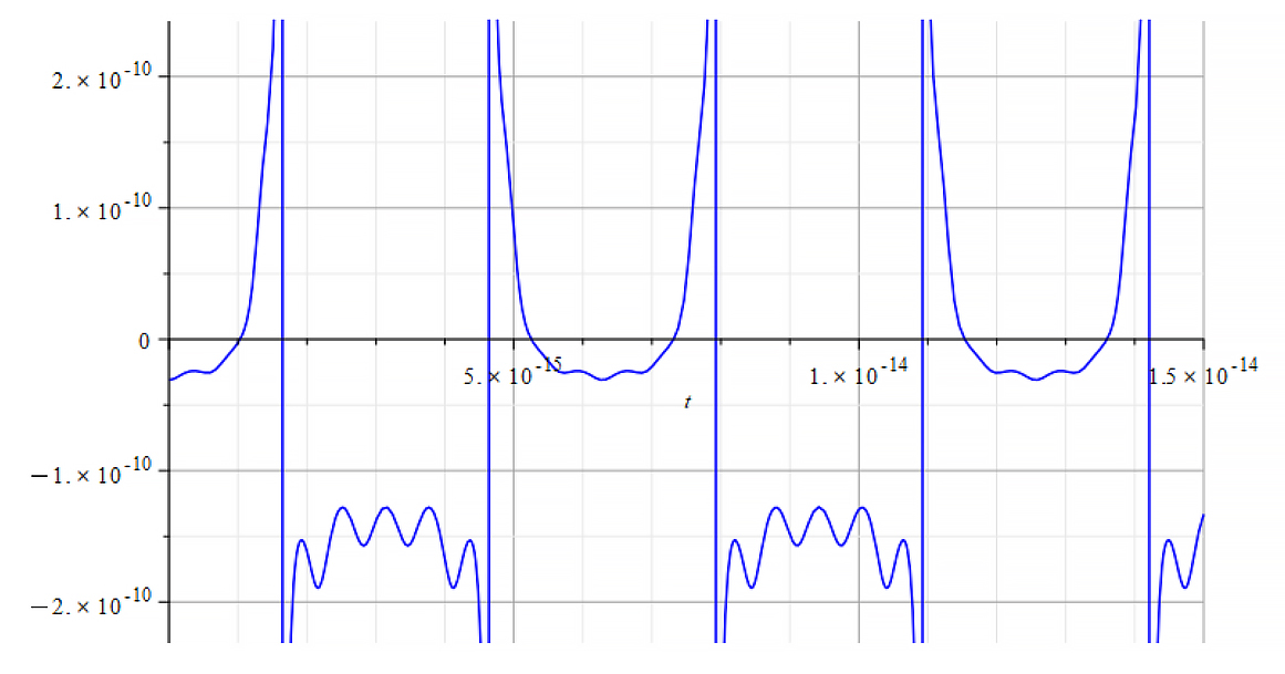
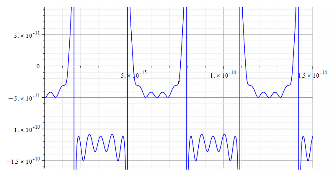
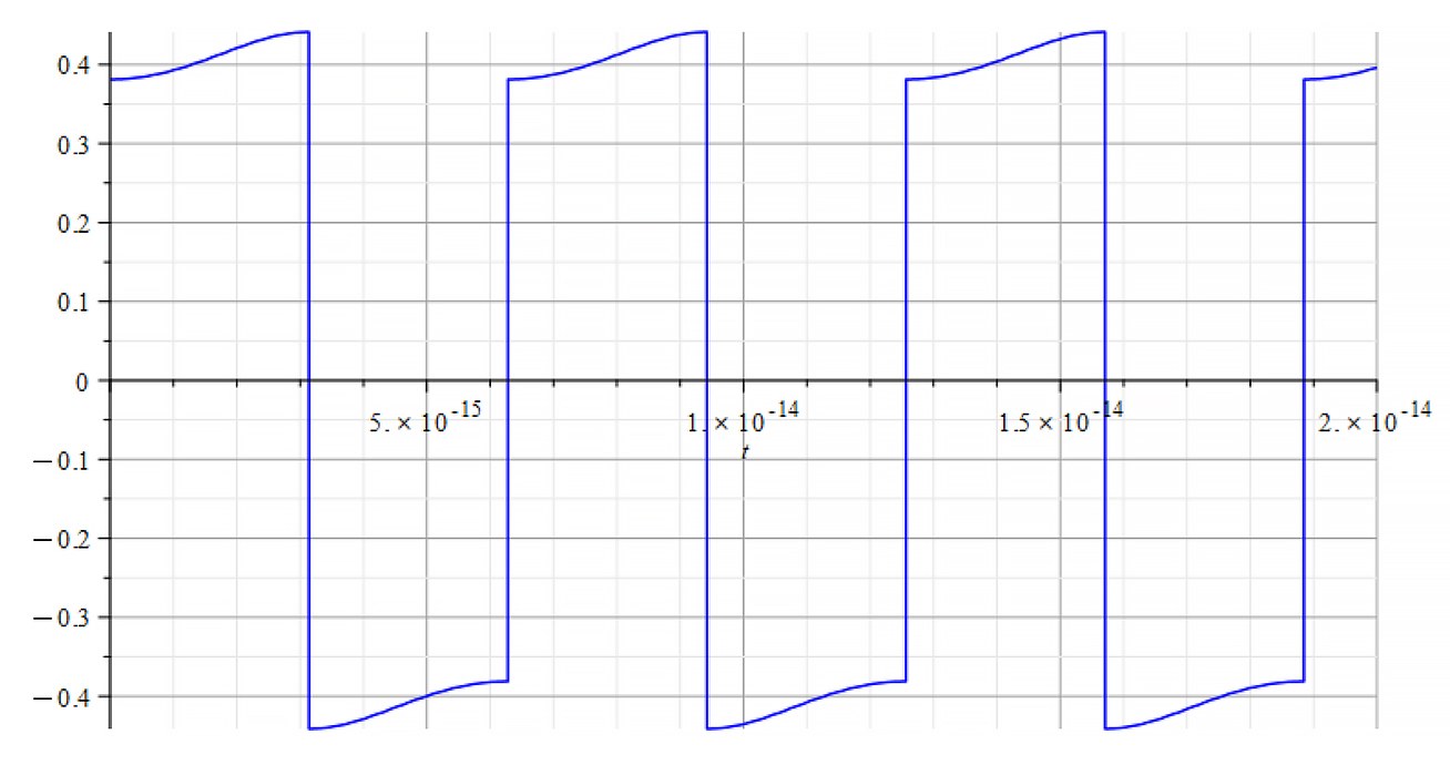
 |  |
| +{E}_{f} Mass vs. time for the following parameters: \omega=1.6\ {10}^{15}\ [\frac{1}{s}]; E_m={10}^{17}\ [\frac{V}{m}]; E_f={10}^{18}\ [\frac{V}{m}] | -{E}_{f} Mass vs. time for the following parameters: \omega=1.6\ {10}^{15}\ [\frac{1}{s}]; E_m={10}^{17}\ [\frac{V}{m}]; E_f={-10}^{18}\ [\frac{V}{m}] |
 |  |
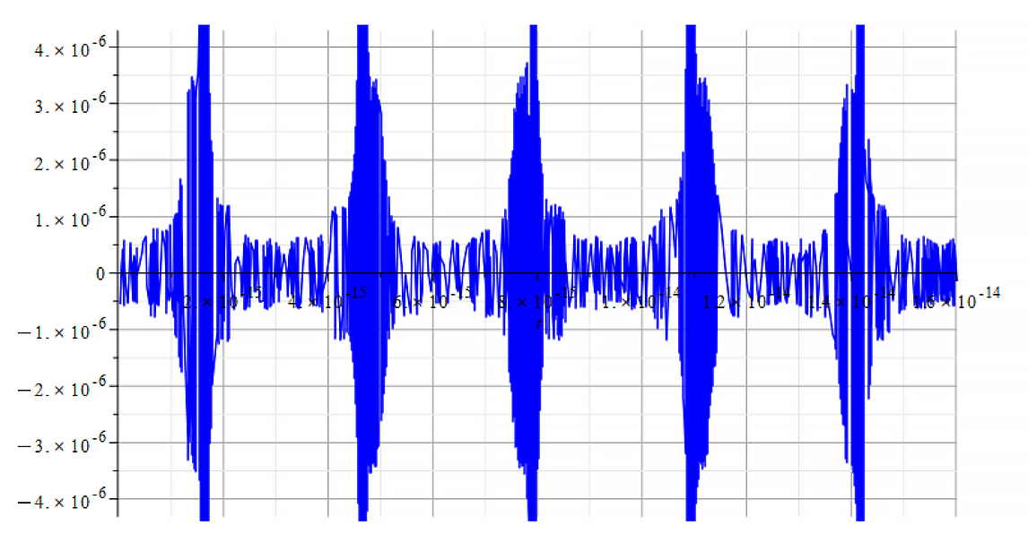
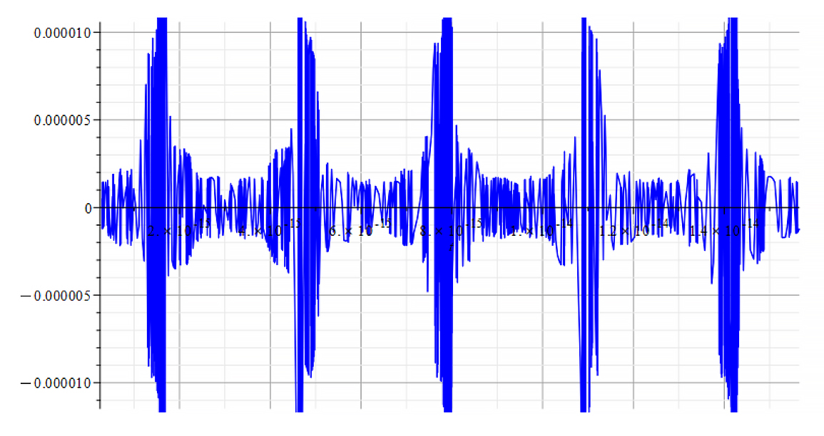
| +{E}_{f} Mass vs. time for the following parameters: \omega={10}^8\ [\frac{1}{s}]; E_m={10}^{15}\ [\frac{V}{m}]; E_f={10}^{17}\ [\frac{V}{m}] | -{E}_{f} Mass vs. time for the following parameters: \omega={10}^8\ [\frac{1}{s}]; E_m={10}^{15}\ [\frac{V}{m}];E_f={-10}^{17}\ [\frac{V}{m}] |
 |  |
| +{E}_{f} Mass vs. time for the following parameters: \omega={10}^{15}\ [\frac{1}{s}]; E_m=7\ {10}^{16}\ [\frac{V}{m}]; E_f={8\ 10}^{17}\ [\frac{V}{m}] | -{E}_{f} Mass vs. time for the following parameters: \omega={10}^{15}\ [\frac{1}{s}]; E_m=7\ {10}^{16}\ [\frac{V}{m}]; E_f={-8\ 10}^{17}\ [\frac{V}{m}] |
From the period of the mass plot, we determine that the oscillation frequency is approximately:
f=1.6\ {10}^{14}\ [Hz]
Frequency Analysis of the Nuclear Mass with FFT
Total number of samples N=2^{13}, sampling frequency f_s=2^3f_p (proton frequency), which gives a frequency resolution \Delta_{f}=\frac{f_s}{N}=1.55\ {10}^{12}[Hz] and a total acquisition time of T=\frac{N}{f_s}=6.43\ {10}^{-13}[s]. The frequency at the i-sample number on the plot is determined by f=\frac{N_{(i)}}{T}\ [Hz].
For +Ef

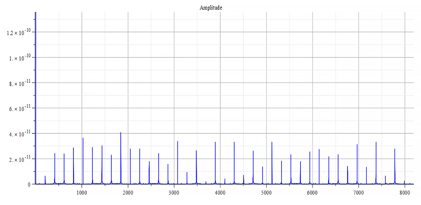
Frequency spectrum for the following parameters: \omega=1.6\ {10}^{15}\ [\frac{1}{s}]; E_m={10}^{17}\ [\frac{V}{m}]; E_f={10}^{18}\ [\frac{V}{m}]
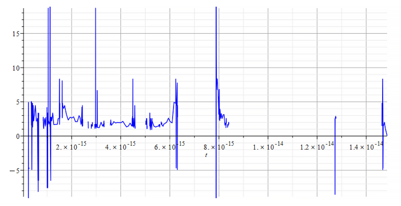
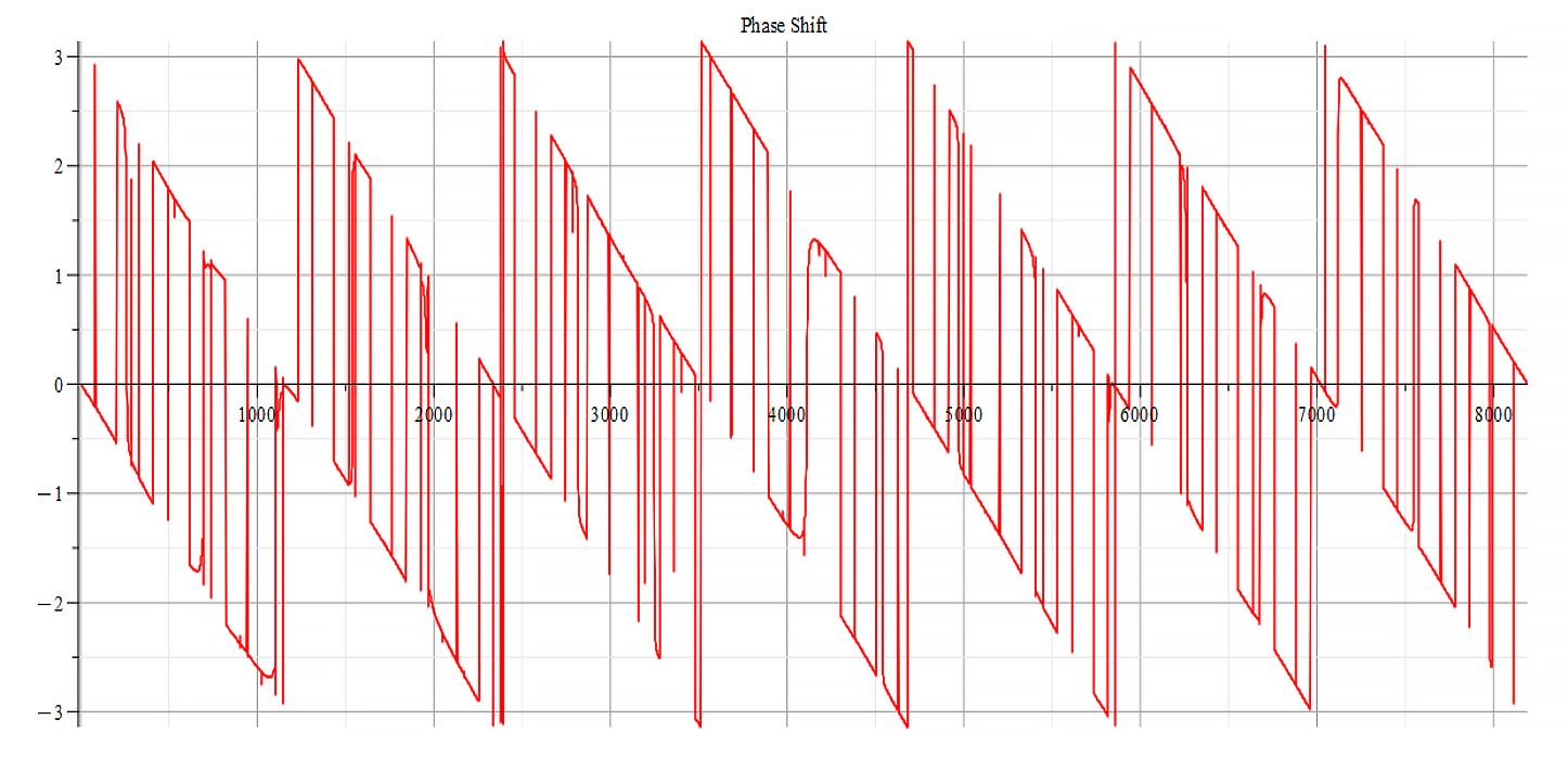
Phase shift for the following parameters: \omega=1.6\ {10}^{15}\ [\frac{1}{s}]; E_m={10}^{17}\ [\frac{V}{m}]; E_f={10}^{18}\ [\frac{V}{m}]
For -Ef
Frequency spectrum for the following parameters: \omega=1.6\ {10}^{15}\ [\frac{1}{s}]; E_m={10}^{17}\ [\frac{V}{m}]; E_f={-10}^{18}\ [\frac{V}{m}]
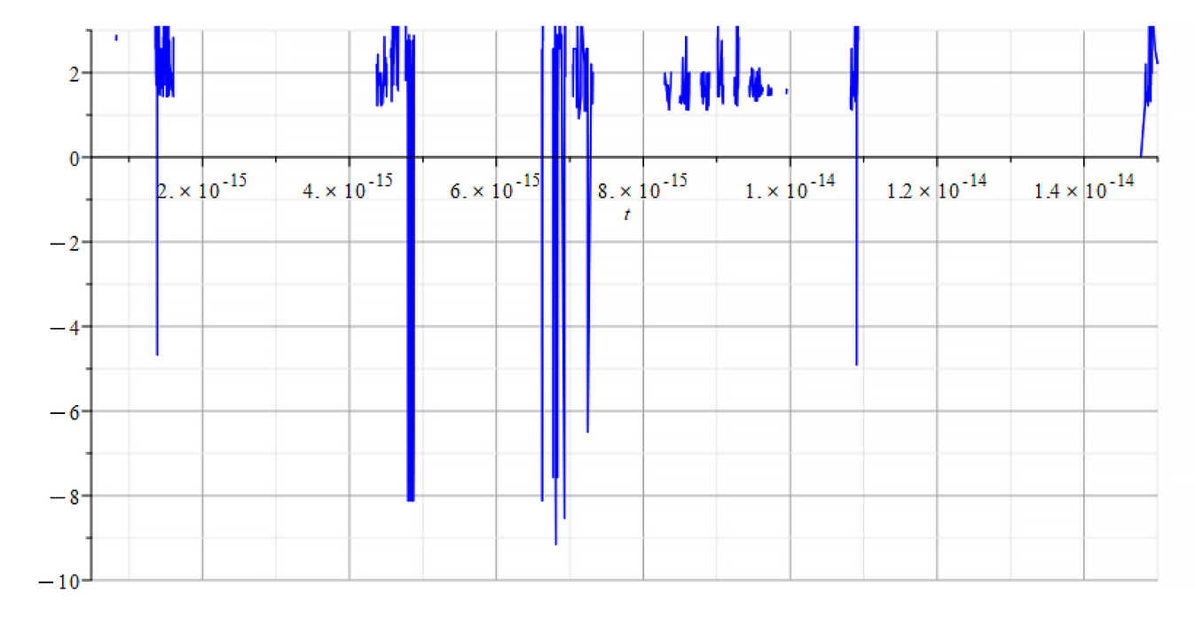
Phase shift for the following parameters: \omega=1.6\ {10}^{15}\ [\frac{1}{s}]; E_m={10}^{17}\ [\frac{V}{m}]; E_f={-10}^{18}\ [\frac{V}{m}]
The frequency spectrum plots are the same. There are some differences in the phase behavior.
From the Fourier frequency analysis, we see that the main frequency is: f_0=1.6\ \ast\ 2\ {10}^{14}\ [Hz].
In general, the main frequency and harmonics is given by the following formula:
f_0=1.6\ \ast\ 2\ {10}^{14}\ [Hz], n=0,\ 1,\ 2,\ 3…
The frequency measured between the first peaks of the double-peak sequence is given by f_n=6.52\ {10}^{13}+n\ \left(f_n-f_{n-1}\right), while the frequency measured between the second peaks of the double-peak sequence is given by f_n=9.63\ {10}^{13}+n\ \left(f_n-f_{n-1}\right).
The frequency gap between peaks on each pair is f_{pp}=1.6\ \ast{2\ 10}^{13}\ [Hz].
For +Ef
Frequency spectrum for the following parameters: \omega={10}^8\ [\frac{1}{s}]; E_m={10}^{15}\ [\frac{V}{m}]; E_f={10}^{17}\ [\frac{V}{m}]
Phase shift for the following parameters: \omega={10}^8\ [\frac{1}{s}]; E_m={10}^{15}\ [\frac{V}{m}]; E_f={10}^{17}\ [\frac{V}{m}]
For -Ef
Frequency spectrum for the following parameters: \omega={10}^8\ [\frac{1}{s}]; E_m={10}^{15}\ [\frac{V}{m}]; E_f={-10}^{17}\ [\frac{V}{m}]
Phase shift for the following parameters: \omega={10}^8\ [\frac{1}{s}]; E_m={10}^{15}\ [\frac{V}{m}]; E_f={-10}^{17}\ [\frac{V}{m}]
The frequency spectrum plots are the same. There are some differences in the phase behavior.
The spectrum contains many frequencies. However, we see that the main frequency is: f_0=1.7\ {10}^{13}\ [Hz].
There is a visible repetition pattern of mirrored three peaks and double peaks.
For +Ef
Frequency spectrum for the following parameters: \omega={10}^{15}\ [\frac{1}{s}]; E_m={7\ 10}^{16}\ [\frac{V}{m}]; E_f={8\ 10}^{17}\ [\frac{V}{m}]
Phase shift for the following parameters: \omega={10}^{15}\ [\frac{1}{s}]; E_m={7\ 10}^{16}\ [\frac{V}{m}]; E_f={8\ 10}^{17}\ [\frac{V}{m}]
For -Ef
Frequency spectrum for the following parameters: \omega={10}^{15}\ [\frac{1}{s}]; E_m={7\ 10}^{16}\ [\frac{V}{m}]; E_f={-8\ 10}^{17}\ [\frac{V}{m}]
Phase shift for the following parameters: \omega={10}^{15}\ [\frac{1}{s}]; E_m={7\ 10}^{16}\ [\frac{V}{m}]; E_f={-8\ 10}^{17}\ [\frac{V}{m}]
The frequency spectrum plots are the same. There are some differences in the phase behavior.
From the Fourier frequency analysis, we see that the main frequency is:
f_0=1.6\ \ast\ 2\ {10}^{14}\ [Hz]
In general, the main frequency and harmonics are given by the following formula:
f_n=f_0+nf_0, n=0,\ 1,\ 2,\ 3…
III.b Refractive Index Analysis due to Force caused by Static Field plus Wave (5) – Total Energy Transmission
When the nucleus is under the action of external forces, and if it doesn’t break apart, then we can assume that a dynamic equilibrium state must exist. Under such circumstances, Newton’s second law requires that the sum of forces be equal to zero, {\vec{F}}{net}+{\vec{F}}{ext}=0, that is,
F_{net}=-F_{ext} (13)
Recall that the net nuclear force has already been written in terms of the index of refraction in Part-1, Eq. (23a):
{\vec{F}}{net}=-\frac{378k q^2}{r{ep}^2\left(t\right)}\left(1-\frac{1}{n^2}+\frac{v_{ep}^2\left(t\right)r_{ep}\left(t\right)a_{ep}\left(t\right)}{n^2c^2}+\frac{1}{n^4}+\frac{2r_{ep}\left(t\right)a_{ep}\left(t\right)}{c^2}\right)\hat{r}+\frac{2279.035793k q^2\hat{r}}{r_n^2}
Now we can equate the forces according to Eq. (13), then solve for “n”,
-\frac{{3.410}^{12}\cdot q^2\left(1-\frac{1}{n^2}+\frac{r_{ep}\left(t\right)a_{ep}\left(t\right)}{n^2c^2}+\frac{1}{n^4}+\frac{2r_{ep}\left(t\right)a_{ep}\left(t\right)}{c^2}\right)}{r_{ep}^2\left(t\right)}+\frac{{2.0510}^{13}\cdot q^2}{r_n^2}=-\frac{\pi\varepsilon_0E_m^2}{6K^3r_n}\cdot\left(2K^3r_n^3+6K^2\cos{\left(\omega t\right)}\sin{\left(\omega t\right)}r_n^2+6K\cos^2{\left(r_nK-\omega t\right)}r_n+6K\sin^2{\left(r_nK-\omega t\right)}r_n-6K\sin^2{\left(\omega t\right)}r_n-6\cos^2{\left(r_nK-\omega t\right)}\omega t-6\sin^2{\left(r_nK-\omega t\right)}\omega t+6\cos^2{\left(\omega t\right)}\omega t+6\sin^2{\left(\omega t\right)}\omega t-3r_nK-3\cos{\left(r_nK-\omega t\right)}\sin{\left(r_nK-\omega t\right)}-3\cos{\left(\omega t\right)}\sin{\left(\omega t\right)}\right)
The refractive index “n” is a somewhat long-expression which is nonsense to copy here. Some plots as examples are shown below, where the main used parameters are:
r_n=3.5\ {10}^{-15}\ [m]; A_e=2\ {10}^{-16}\ [m]; A_p={10}^{-3}A_e\ [m]; N_0=378; N_s=312
\omega_e={10}^{15}\ [\frac{1}{s}]; \omega_p={10}^{16}\ [\frac{1}{s}]
While for the wave: K=\frac{\omega}{c}
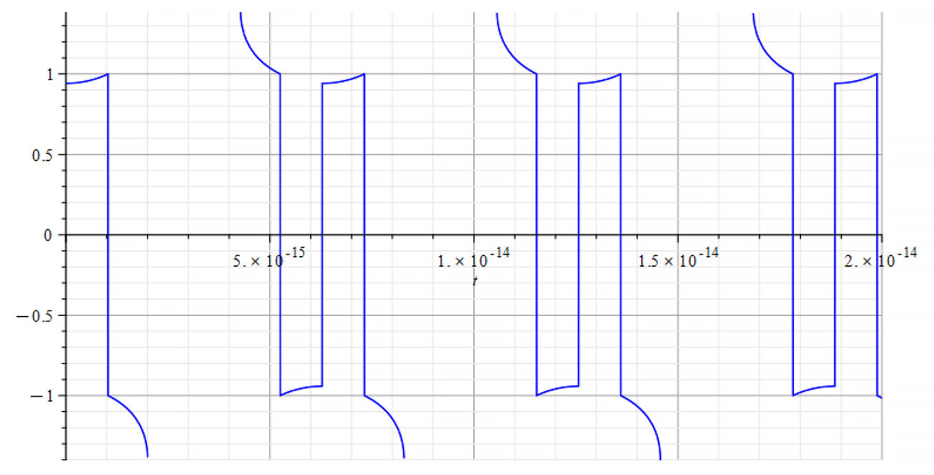
 |  |
| +{E}_{f} Refractive Index vs. time for the following parameters: \omega=1.6\ {10}^{15}\ [\frac{1}{s}]; E_m={10}^{17}\ [\frac{V}{m}]; E_f={10}^{18}\ [\frac{V}{m}] | -{E}_{f} Refractive Index vs. time for the following parameters: \omega=1.6\ {10}^{15}\ [\frac{1}{s}]; E_m={10}^{17}\ [\frac{V}{m}]; E_f={-10}^{18}\ [\frac{V}{m}] |
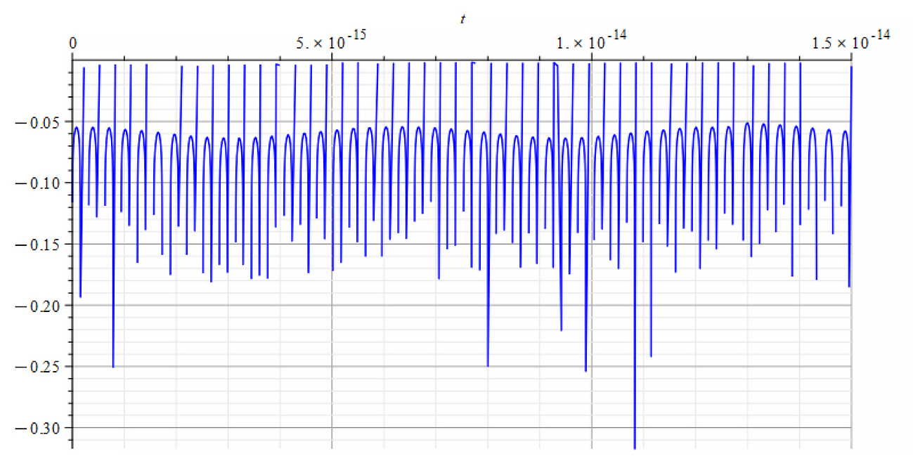
 |  |
| +{E}_{f} Refractive Index vs. time for the following parameters: \omega={10}^8\ [\frac{1}{s}]; E_m={10}^{15}\ [\frac{V}{m}]; E_f={10}^{17}\ [\frac{V}{m}] | -{E}_{f} Refractive Index vs. time for the following parameters: \omega={10}^8\ [\frac{1}{s}]; E_m={10}^{15}\ [\frac{V}{m}]; E_f={-10}^{17}\ [\frac{V}{m}] |
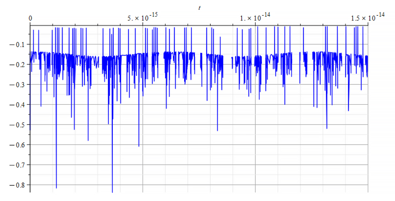
 |  |
| +{E}_{f} Refractive Index vs. time for the following parameters: \omega={10}^{15}\ [\frac{1}{s}]; E_m=7\ {10}^{16}\ [\frac{V}{m}]; E_f={8\ 10}^{17}\ [\frac{V}{m}] | -{E}_{f} Refractive Index vs. time for the following parameters: \omega={10}^{15}\ [\frac{1}{s}]; E_m=7\ {10}^{16}\ [\frac{V}{m}]; E_f={-8\ 10}^{17}\ [\frac{V}{m}] |
The refractive index derived from the integration that gave force (5) shows bizarre values and might not be considered as valid in this case. It is also possible that the graph engine threw such unreal values at asymptotic points due to the extreme oscillatory behavior of the mass in these cases.
III.c Comparison of Mass with Refractive Index Behavior due to Force caused by Static Field plus Wave (5) – Total Energy Transmission
To analyze the changes in the refractive index “n” with respect to changes in nuclear mass, overlaid graphs of both quantities are shown below, which uncover interesting results.
While for the wave: K=\frac{\omega}{c}
 |  |
| +{E}_{f} Mass & Refractive Index vs. time for the following parameters: \omega=1.6\ {10}^{15}\ [\frac{1}{s}]; E_m={10}^{17}\ [\frac{V}{m}]; E_f={10}^{18}\ [\frac{V}{m}] | -{E}_{f} Mass & Refractive Index vs. time for the following parameters: \omega=1.6\ {10}^{15}\ [\frac{1}{s}]; E_m={10}^{17}\ [\frac{V}{m}]; E_f={-10}^{18}\ [\frac{V}{m}] |
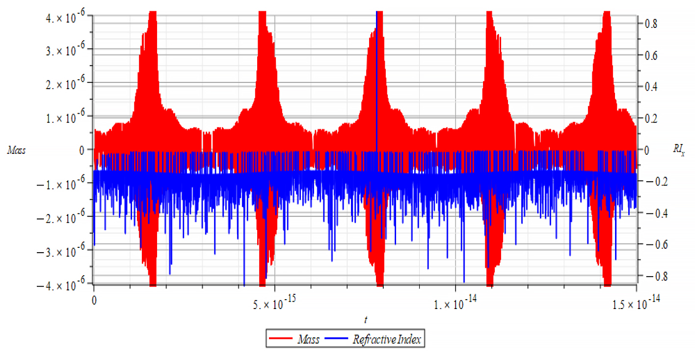
 |  |
| +{E}_{f} Mass & Refractive Index vs. time for the following parameters: \omega={10}^8\ [\frac{1}{s}]; E_m={10}^{15}\ [\frac{V}{m}]; E_f={10}^{17}\ [\frac{V}{m}] | -{E}_{f} Mass & Refractive Index vs. time for the following parameters: \omega={10}^8\ [\frac{1}{s}]; E_m={10}^{15}\ [\frac{V}{m}]; E_f={-10}^{17}\ [\frac{V}{m}] |
 |  |
| +{E}_{f} Mass & Refractive Index vs. time for the following parameters: \omega={10}^{15}\ [\frac{1}{s}]; E_m=7\ {10}^{16}\ [\frac{V}{m}]; E_f={8\ 10}^{17}\ [\frac{V}{m}] | -{E}_{f} Mass & Refractive Index vs. time for the following parameters: \omega={10}^{15}\ [\frac{1}{s}]; E_m=7\ {10}^{16}\ [\frac{V}{m}]; E_f={-8\ 10}^{17}\ [\frac{V}{m}] |
As stated in the previous paragraph, it is impossible to make any comparison between mass and refractive index in these cases, because the high-frequency oscillations of the mass yield very sharp changes in the refractive index. As a result, it is highly probable that the graph engine can’t follow such changes the right way.
IV.a Nuclear Mass Analysis due to Force caused by Static Field plus Wave (6) – Energy Absorption/Transmission
The intrinsic net force in the nucleus was already defined with Eq. (23) in Part-1. Now we have the action of an external force acting on the nucleus that will interact with the internal force. By applying Newton’s second law, we have
\sum F=m_n\cdot a_{ep}=F_{net}+F_{ext} => m_n\cdot a_{ep}=F_{net}+F_{ext}
m_n=\frac{1}{a_{ep}}\cdot\left(F_{net}+F_{ext}\right) (14)
By replacing the forces in (14), we obtain the expression of the nuclear mass for this case:
m_n=\frac{1}{a_{ep}\left(t\right)}\cdot\left(-\frac{{3.410}^{12}\cdot q^2\left(1-\frac{v_{ep}^2\left(t\right)}{c^2}+\frac{v_{ep}^2\left(t\right)r_{ep}\left(t\right)a_{ep}\left(t\right)}{c^4}+\frac{v_{ep}^4\left(t\right)}{c^4}+\frac{2r_{ep}\left(t\right)a_{ep}\left(t\right)}{c^2}\right)}{r_{ep}^2\left(t\right)}+\frac{{2.0510}^{13}\cdot q^2}{r_n^2}+\frac{2\varepsilon_0\omega}{3c K^3}\cdot\left(-\frac{3E_m^2\sin{\left(2Kr_n-2\omega t\right)}}{8}-12E_fE_m\sin{\left(Kr_n-\omega t\right)}+\frac{3\left(K^2r_n^2-\frac{1}{2}\right)E_m^2\sin{\left(2\omega t\right)}}{4}+\frac{3E_m^2r_nK\cos{\left(2\omega t\right)}}{4}+6E_fE_m\left(K^2r_n^2-2\right)\sin{\left(\omega t\right)}+r_n\left(12E_fE_m\cos{\left(\omega t\right)}+K^2r_n^2\left(E_f^2+\frac{E_m^2}{2}\right)\right)K\right)\right) (15)
Recall that:
r_{ep}\left(t\right)=\left(0.37r_n+A_e\cos{\left(\omega_et\right)}-A_p\cos{\left(\omega_pt\right)}\right)
v_{ep}\left(t\right)=\left(-A_e\omega_e\sin{\left(\omega_et\right)}+A_p\sin{\left(\omega_pt\right)}\omega_p\right)
a_{ep}\left(t\right)=\left(-A_e\omega_e^2\cos{\left(\omega_et\right)}+A_p\omega_p^2\cos{\left(\omega_pt\right)}\right)
Some graphs as examples are shown below to have a perception of what could be done to modify the nuclear mass magnitude and sign.
The main parameters used for the net force are:
r_n=3.5\ {10}^{-15}\ [m]; A_e=2\ {10}^{-16}\ [m]; A_p={10}^{-3}A_e\ [m]; N_0=378; N_s=312
\omega_e={10}^{15}\ [\frac{1}{s}]; \omega_p={10}^{16}\ [\frac{1}{s}]
While for the wave: K=\frac{\omega}{c} and K=\frac{\omega}{v_{ep}\left(t\right)}
Time Analysis of the Nuclear Mass for Wave Velocity “c” and “vep(t)” and electric field polarity ± Ef
For +Ef
 |  |
| K=\frac{\omega}{c} Mass vs. time for the following parameters: \omega=6\ {10}^{14}\ [\frac{1}{s}]; E_m={10}^{26}\ [\frac{V}{m}]; E_f=3\ {10}^{27}\ [\frac{V}{m}] | K=\frac{\omega}{v_{ep}\left(t\right)} Mass vs. time for the following parameters: \omega=6\ {10}^{14}\ [\frac{1}{s}]; E_m={10}^{26}\ [\frac{V}{m}]; E_f=3\ {10}^{27}\ [\frac{V}{m}] |
For -Ef
 |  |
| K=\frac{\omega}{c} Mass vs. time for the following parameters: \omega=6\ {10}^{14}\ [\frac{1}{s}]; E_m={10}^{24}\ [\frac{V}{m}]; E_f=-1.5\ {10}^{26}\ [\frac{V}{m}] | K=\frac{\omega}{v_{ep}\left(t\right)} Mass vs. time for the following parameters: \omega=6\ {10}^{14}\ [\frac{1}{s}]; E_m={10}^{24}\ [\frac{V}{m}]; E_f=-1.5\ {10}^{26}\ [\frac{V}{m}] |
For +Ef
 |  |
| K=\frac{\omega}{c} Mass vs. time for the following parameters: \omega=2\ {10}^{16}\ [\frac{1}{s}]; E_m=8\ {10}^{25}\ [\frac{V}{m}]; E_f={3\ 10}^{26}\ [\frac{V}{m}] | K=\frac{\omega}{v_{ep}\left(t\right)} Mass vs. time for the following parameters: \omega=2\ {10}^{16}\ [\frac{1}{s}]; E_m=8\ {10}^{25}\ [\frac{V}{m}]; E_f={3\ 10}^{26}\ [\frac{V}{m}] |
For -Ef
 |  |
| K=\frac{\omega}{c} Mass vs. time for the following parameters: \omega=2\ {10}^{16}\ [\frac{1}{s}]; E_m={10}^{24}\ [\frac{V}{m}]; E_f={-10}^{25}\ [\frac{V}{m}] | K=\frac{\omega}{v_{ep}\left(t\right)} Mass vs. time for the following parameters: \omega=2\ {10}^{16}\ [\frac{1}{s}]; E_m={10}^{24}\ [\frac{V}{m}]; E_f={-10}^{25}\ [\frac{V}{m}] |
For +Ef
 |  |
| K=\frac{\omega}{c} Mass vs. time for the following parameters: \omega={10}^{18}\ [\frac{1}{s}]; E_m={10}^{23}\ [\frac{V}{m}]; E_f=2.5\ {10}^{24}\ [\frac{V}{m}] | K=\frac{\omega}{v_{ep}\left(t\right)} Mass vs. time for the following parameters: \omega={10}^{18}\ [\frac{1}{s}]; E_m={10}^{23}\ [\frac{V}{m}]; E_f=2.5\ {10}^{24}\ [\frac{V}{m}] |
For -Ef
 |  |
| K=\frac{\omega}{c} Mass vs. time for the following parameters: \omega={10}^{18}\ [\frac{1}{s}]; E_m={10}^{23}\ [\frac{V}{m}]; E_f={-7\ 10}^{24}\ [\frac{V}{m}] | K=\frac{\omega}{v_{ep}\left(t\right)} Mass vs. time for the following parameters: \omega={10}^{18}\ [\frac{1}{s}]; E_m={10}^{23}\ [\frac{V}{m}]; E_f={-7\ 10}^{24}\ [\frac{V}{m}] |
From the period of the mass plot, we determine that the oscillation frequency is approximately:
f=1.6\ {10}^{14}\ [Hz]
Frequency Analysis of the Nuclear Mass with FFT for Wave Velocity “c” and Electric Field Polarity ± Ef
Total number of samples N=2^{14}\ or{\ 2}^{15}, sampling frequency f_s\geq2^3f_w (wave frequency), which gives a frequency resolution \Delta_{f}=\frac{f_s}{N}[Hz] and a total acquisition time of T=\frac{N}{f_s}[s]. The frequency at the i-sample number on the plot is determined by f=\frac{N_{(i)}}{T}\ [Hz].
For +Ef
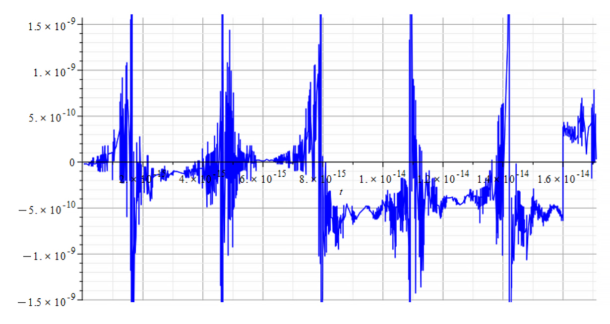
 |  |
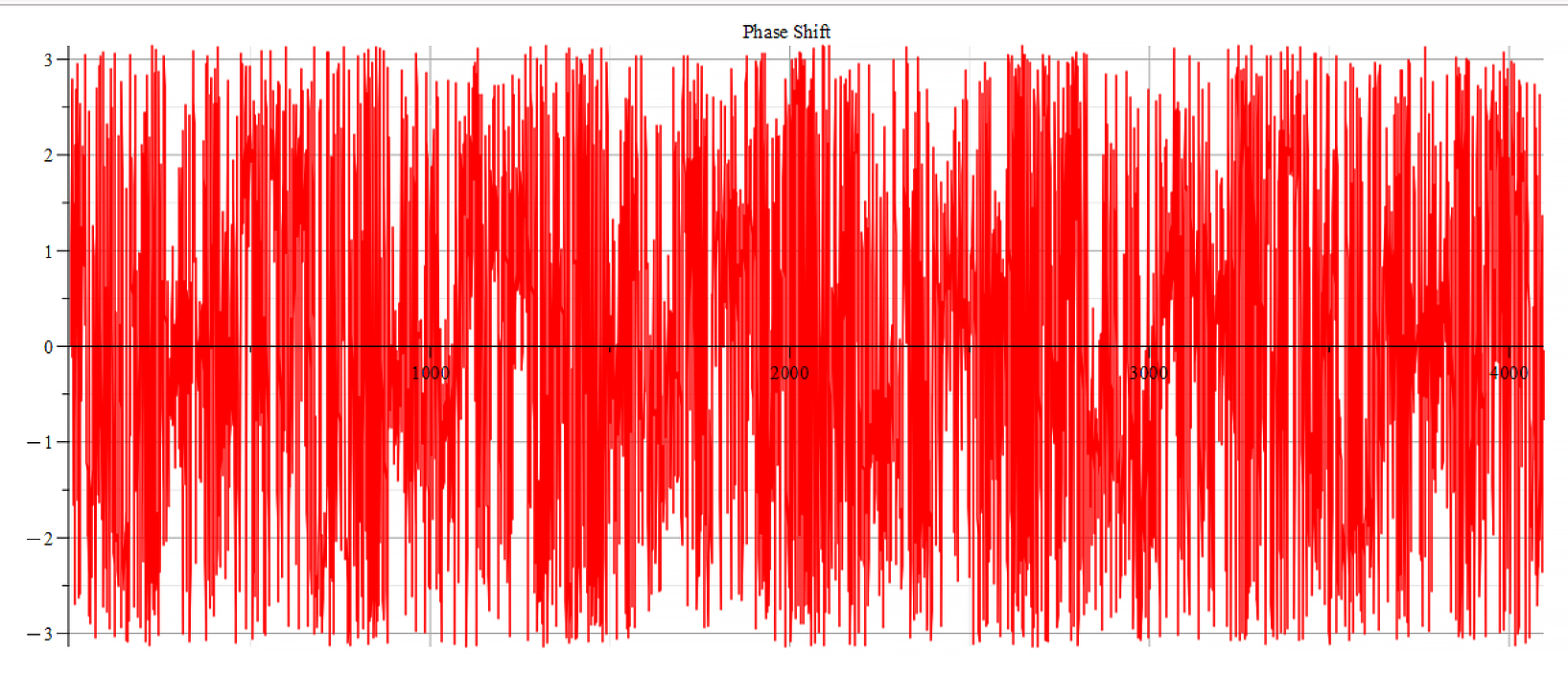
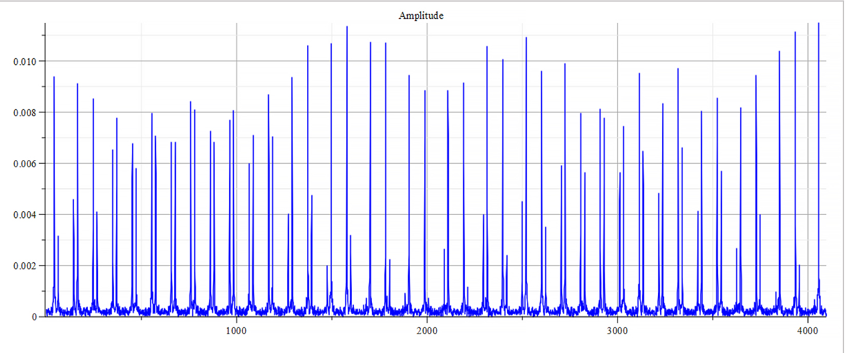
| Frequency spectrum for the following parameters: \omega=6\ {10}^{14}\ [\frac{1}{s}]; E_m={10}^{26}\ [\frac{V}{m}]; E_f=3\ {10}^{27}\ [\frac{V}{m}] | Phase shift for the same parameters |
Fig. 49
For -Ef
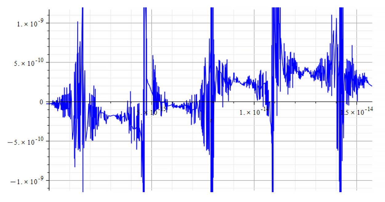
 |  |
| Frequency spectrum for the following parameters: \omega=6\ {10}^{14}\ [\frac{1}{s}]; E_m={10}^{24}\ [\frac{V}{m}]; E_f=-1.5\ {10}^{26}\ [\frac{V}{m}] | Phase shift for the same parameters |
Fig. 50
Both frequency spectrum plots are very similar, but phase behavior differs. The spectrum contains many frequencies, being the main measured at the small amplitudes near the origin to be: f_0=2.33\ {10}^{12}\ [Hz]. In general, the main frequency and harmonics are given by the following formula: f_n=f_0+nf_0, n=0,\ 1,\ 2,\ 3…, and for this case,
f_n=2.33\ {10}^{12}+n\ {7\ 10}^{12}\ [Hz].
There is a visible repetition pattern of high amplitude mirrored double peaks which repeat periodically. However, it’s somewhat difficult to determine the repetition frequency.
For +Ef
 |  |
| Frequency spectrum for the following parameters: \omega=2\ {10}^{16}\ [\frac{1}{s}]; E_m=8\ {10}^{25}\ [\frac{V}{m}]; E_f=3\ {10}^{26}\ [\frac{V}{m}] | Phase shift for the same parameters |
Fig. 51
For -Ef
 |  |
| Frequency spectrum for the following parameters: \omega=2\ {10}^{16}\ [\frac{1}{s}]; E_m={10}^{24}\ [\frac{V}{m}]; E_f=-{10}^{25}\ [\frac{V}{m}] | Phase shift for the same parameters |
Fig. 52
Both frequency spectrum plots are very similar, but phase behavior differs. The spectrum contains many frequencies, but by measuring the high amplitude peaks we get the main frequency to be: f_0=2\ \ast\ 1.6\ {10}^{14}\ [Hz]. In general, the main frequency and harmonics are given by the following formula: f_n=f_0+nf_0, n=0,\ 1,\ 2,\ 3…, and for this case,
f_n=2\ \ast1.6\ {10}^{14}+n\ 2\ \ast\ 1.6\ {10}^{14}\ [Hz].
For +Ef
 |  |
| Frequency spectrum for the following parameters: \omega={10}^{18}\ [\frac{1}{s}]; E_m={10}^{23}\ [\frac{V}{m}]; E_f=2.5\ {10}^{24}\ [\frac{V}{m}] | Phase shift for the same parameters |
Fig. 53
For +Ef (expanded)
 |  |
| Frequency spectrum for the following parameters: \omega={10}^{18}\ [\frac{1}{s}]; E_m={10}^{23}\ [\frac{V}{m}]; E_f=2.5\ {10}^{24}\ [\frac{V}{m}] | Phase shift for the same parameters |
Fig. 54
For -Ef
 |  |
| Frequency spectrum for the following parameters: \omega={10}^{18}\ [\frac{1}{s}]; E_m={10}^{23}\ [\frac{V}{m}]; E_f=-7\ {10}^{24}\ [\frac{V}{m}] | Phase shift for the same parameters |
Fig. 55
For -Ef (expanded)
 |  |
| Frequency spectrum for the following parameters: \omega={10}^{18}\ [\frac{1}{s}]; E_m={10}^{23}\ [\frac{V}{m}]; E_f=-7\ {10}^{24}\ [\frac{V}{m}] | Phase shift for the same parameters |
Fig. 56
Both frequency spectrum plots are very similar, but phase behavior differs. The spectrum contains many frequencies, but by measuring the high amplitude peaks, we get the main frequency to be: f_0=3.5\ {10}^{14}\ [Hz]. In general, the main frequency and harmonics are given by the following formula: f_n=f_0+nf_0, n=0,\ 1,\ 2,\ 3…, and for this case,
f_n=3.5\ {10}^{14}+n\ 3.1\ {10}^{14}\ [Hz].
Frequency Analysis of the Nuclear Mass with FFT for Wave Velocity “vep(t)” and Electric Field Polarity ± Ef
Total number of samples N=2^{14}\ or{\ 2}^{15}, sampling frequency f_s\geq2^3f_w (wave frequency), which gives a frequency resolution \Delta_{f}=\frac{f_s}{N}[Hz] and a total acquisition time of T=\frac{N}{f_s}[s]. The frequency at the i-sample number on the plot is determined by f=\frac{N_{(i)}}{T}\ [Hz].
For +Ef
 |  |
| Frequency spectrum for the following parameters: \omega=6\ {10}^{14}\ [\frac{1}{s}]; E_m={10}^{26}\ [\frac{V}{m}]; E_f=3\ {10}^{27}\ [\frac{V}{m}] | Phase shift for the same parameters |
Fig. 57
For -Ef
 |  |
| Frequency spectrum for the following parameters: \omega=6\ {10}^{14}\ [\frac{1}{s}]; E_m={10}^{24}\ [\frac{V}{m}]; E_f=-1.5\ {10}^{26}\ [\frac{V}{m}] | Phase shift for the same parameters |
Fig. 58
We get the main frequency to be: f_0=1.6\ {10}^{14}\ [Hz]. In general, the main frequency and harmonics are given by the following formula: f_n=f_0+nf_0, n=0,\ 1,\ 2,\ 3…
For +Ef
 |  |
| Frequency spectrum for the following parameters: \omega=2\ {10}^{16}\ [\frac{1}{s}]; E_m=8\ {10}^{25}\ [\frac{V}{m}]; E_f=3\ {10}^{26}\ [\frac{V}{m}] | Phase shift for the same parameters |
Fig. 59
For -Ef
 |  |
| Frequency spectrum for the following parameters: \omega=2\ {10}^{16}\ [\frac{1}{s}]; E_m={10}^{24}\ [\frac{V}{m}]; E_f=-{10}^{25}\ [\frac{V}{m}] | Phase shift for the same parameters |
Fig. 60
We get the main frequency to be: f_0=1.6\ {10}^{14}\ [Hz]. In general, the main frequency and harmonics are given by the following formula: f_n=f_0+nf_0, n=0,\ 1,\ 2,\ 3…
For +Ef
 |  |
| Frequency spectrum for the following parameters: \omega={10}^{18}\ [\frac{1}{s}]; E_m={10}^{23}\ [\frac{V}{m}]; E_f=2.5\ {10}^{24}\ [\frac{V}{m}] | Phase shift for the same parameters |
Fig. 61
For +Ef (expanded)
 |  |
| Frequency spectrum for the following parameters: \omega={10}^{18}\ [\frac{1}{s}]; E_m={10}^{23}\ [\frac{V}{m}]; E_f=2.5\ {10}^{24}\ [\frac{V}{m}] | Phase shift for the same parameters |
Fig. 62
For -Ef
 |  |
| Frequency spectrum for the following parameters: \omega={10}^{18}\ [\frac{1}{s}]; E_m={10}^{23}\ [\frac{V}{m}]; E_f=-7\ {10}^{24}\ [\frac{V}{m}] | Phase shift for the same parameters |
Fig. 63
Expanded graphs for -Ef look like those for +Ef.
We get the main frequency to be: f_0=3.8\ {10}^{14}\ [Hz]. In general, the main frequency and harmonics are given by the following formula: f_n=f_0+nf_0, n=0,\ 1,\ 2,\ 3…, and for this case,
f_n=3.8\ {10}^{14}+n\ \ast\ 2\ \ast\ 1.6\ {10}^{14}\ [Hz].
IV.b Refractive Index Analysis due to Wave Force (6) for Wave Velocity “c” and “vep(t)” and Electric Field Polarity ± Ef
When the nucleus is under the action of external forces, and if it doesn’t break apart, then we can assume that a dynamic equilibrium state must exist. Under such circumstances, Newton’s second law requires that the sum of forces be equal to zero, {\vec{F}}{net}+{\vec{F}}{ext}=0, that is,
F_{net}=-F_{ext} (16)
Recall that the net nuclear force has already been written in terms of the index of refraction in Part-1, Eq. (23a):
{\vec{F}}{net}=-\frac{378k q^2}{r{ep}^2\left(t\right)}\left(1-\frac{1}{n^2}+\frac{v_{ep}^2\left(t\right)r_{ep}\left(t\right)a_{ep}\left(t\right)}{n^2c^2}+\frac{1}{n^4}+\frac{2r_{ep}\left(t\right)a_{ep}\left(t\right)}{c^2}\right)\hat{r}+\frac{2279.035793k q^2\hat{r}}{r_n^2}
Now we can equate the forces according to Eq. (16), then solve for “n”,
-\frac{{3.410}^{12}\cdot q^2\left(1-\frac{1}{n^2}+\frac{r_{ep}\left(t\right)a_{ep}\left(t\right)}{n^2c^2}+\frac{1}{n^4}+\frac{2r_{ep}\left(t\right)a_{ep}\left(t\right)}{c^2}\right)}{r_{ep}^2\left(t\right)}+\frac{{2.0510}^{13}\cdot q^2}{r_n^2}=-\frac{2\varepsilon_0\omega}{3c K^3}\cdot\left(-\frac{3E_m^2\sin{\left(2Kr_n-2\omega t\right)}}{8}-12E_fE_m\sin{\left(Kr_n-\omega t\right)}+\frac{3\left(K^2r_n^2-\frac{1}{2}\right)E_m^2\sin{\left(2\omega t\right)}}{4}+\frac{3E_m^2r_nK\cos{\left(2\omega t\right)}}{4}+6E_fE_m\left(K^2r_n^2-2\right)\sin{\left(\omega t\right)}+r_n\left(12E_fE_m\cos{\left(\omega t\right)}+K^2r_n^2\left(E_f^2+\frac{E_m^2}{2}\right)\right)K\right)
The refractive index “n” is a somewhat long-expression which is nonsense to copy here. Some plots as examples are shown below, where the main used parameters are:
r_n=3.5\ {10}^{-15}\ [m]; A_e=2\ {10}^{-16}\ [m]; A_p={10}^{-3}A_e\ [m]; N_0=378; N_s=312
\omega_e={10}^{15}\ [\frac{1}{s}]; \omega_p={10}^{16}\ [\frac{1}{s}]
While for the wave: K=\frac{\omega}{c} and K=\frac{\omega}{v_{ep}\left(t\right)}
For +Ef
 |  |
| K=\frac{\omega}{c} Refractive Index vs. time for the following parameters: \omega=6\ {10}^{14}\ [\frac{1}{s}]; E_m={10}^{26}\ [\frac{V}{m}]; E_f=3\ {10}^{27}\ [\frac{V}{m}] | K=\frac{\omega}{v_{ep}\left(t\right)} Refractive Index vs. time for the following parameters: \omega=6\ {10}^{14}\ [\frac{1}{s}]; E_m={10}^{26}\ [\frac{V}{m}]; E_f=3\ {10}^{27}\ [\frac{V}{m}] |
For -Ef
 |  |
| K=\frac{\omega}{c} Refractive Index vs. time for the following parameters: \omega=6\ {10}^{14}\ [\frac{1}{s}]; E_m={10}^{24}\ [\frac{V}{m}]; E_f=-1.5\ {10}^{26}\ [\frac{V}{m}] | K=\frac{\omega}{v_{ep}\left(t\right)} Refractive Index vs. time for the following parameters: \omega=6\ {10}^{14}\ [\frac{1}{s}]; E_m={10}^{24}\ [\frac{V}{m}]; E_f=-1.5\ {10}^{26}\ [\frac{V}{m}] |
For +Ef
 |  |
| K=\frac{\omega}{c} Refractive Index vs. time for the following parameters: \omega=2\ {10}^{16}\ [\frac{1}{s}]; E_m=8\ {10}^{25}\ [\frac{V}{m}]; E_f={3\ 10}^{26}\ [\frac{V}{m}] | K=\frac{\omega}{v_{ep}\left(t\right)} Refractive Index vs. time for the following parameters: \omega=2\ {10}^{16}\ [\frac{1}{s}]; E_m=8\ {10}^{25}\ [\frac{V}{m}]; E_f={3\ 10}^{26}\ [\frac{V}{m}] |
For -Ef
 |  |
| K=\frac{\omega}{c} Refractive Index vs. time for the following parameters: \omega=2\ {10}^{16}\ [\frac{1}{s}]; E_m={10}^{24}\ [\frac{V}{m}]; E_f={-10}^{25}\ [\frac{V}{m}] | K=\frac{\omega}{v_{ep}\left(t\right)} Refractive Index vs. time for the following parameters: \omega=2\ {10}^{16}\ [\frac{1}{s}]; E_m={10}^{24}\ [\frac{V}{m}]; E_f={-10}^{25}\ [\frac{V}{m}] |
For +Ef
 |  |
| K=\frac{\omega}{c} Refractive Index vs. time for the following parameters: \omega={10}^{18}\ [\frac{1}{s}]; E_m={10}^{23}\ [\frac{V}{m}]; E_f=2.5\ {10}^{24}\ [\frac{V}{m}] | K=\frac{\omega}{v_{ep}\left(t\right)} Refractive Index vs. time for the following parameters: \omega={10}^{18}\ [\frac{1}{s}]; E_m={10}^{23}\ [\frac{V}{m}]; E_f=2.5\ {10}^{24}\ [\frac{V}{m}] |
For -Ef
 |  |
| K=\frac{\omega}{c} Refractive Index vs. time for the following parameters: \omega={10}^{18}\ [\frac{1}{s}]; E_m={10}^{23}\ [\frac{V}{m}];E_f={-7\ 10}^{24}\ [\frac{V}{m}] | K=\frac{\omega}{v_{ep}\left(t\right)} Refractive Index vs. time for the following parameters: \omega={10}^{18}\ [\frac{1}{s}]; E_m={10}^{23}\ [\frac{V}{m}]; E_f={-7\ 10}^{24}\ [\frac{V}{m}] |
We observe that for wave velocity “c”, under the given conditions, the refractive index is negative in most of the cases.
IV.c Comparison of Mass with Refractive Index Behavior due to Force caused by Static Field plus Wave (6), for Wave Velocity “c” and “vep(t)” and ± Ef
To analyze the changes in the refractive index “n” with respect to changes in nuclear mass, overlaid graphs of both quantities are shown below, which uncover interesting results.
For +Ef
 |  |
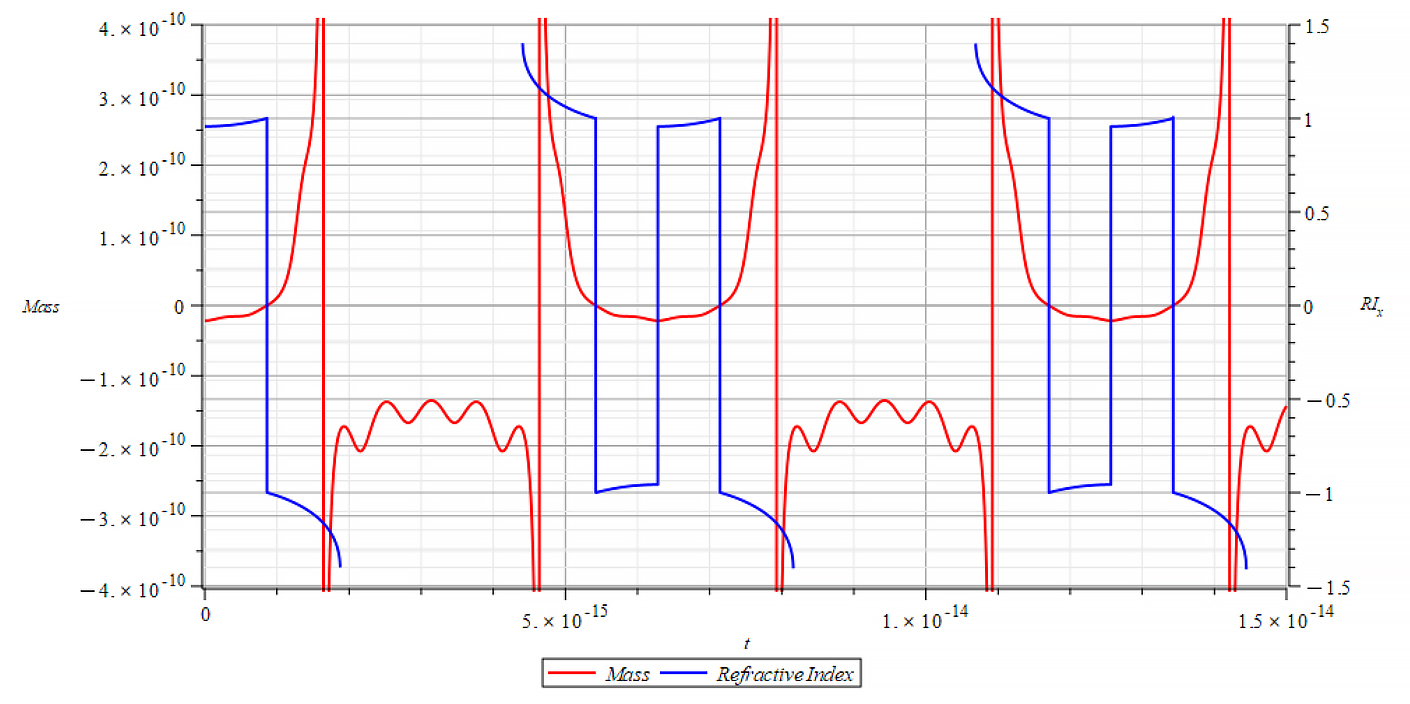
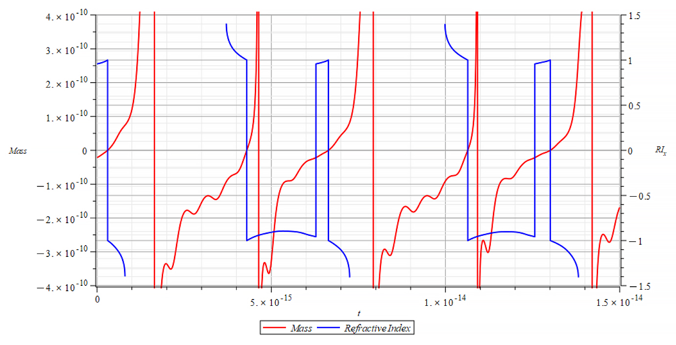
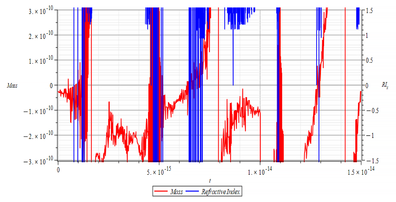
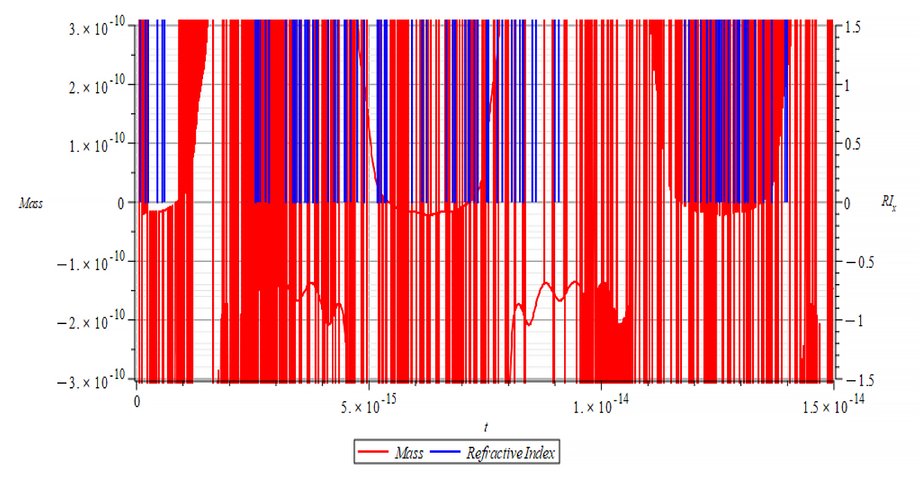
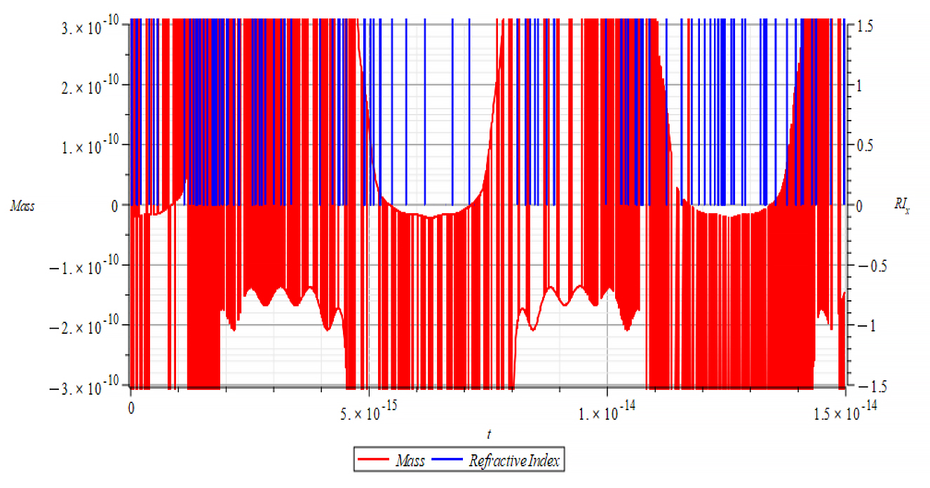
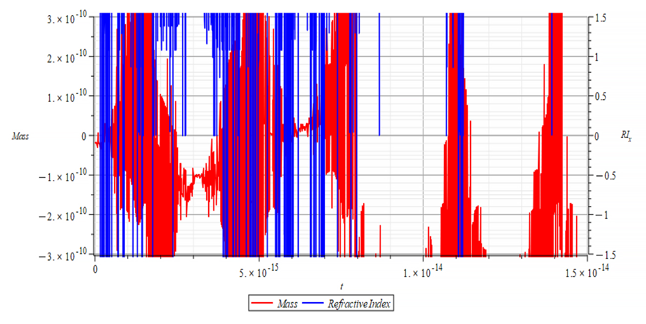
| K=\frac{\omega}{c} Mass & Refractive Index vs. time for the following parameters: \omega=6\ {10}^{14}\ [\frac{1}{s}]; E_m={10}^{26}\ [\frac{V}{m}]; E_f=3\ {10}^{27}\ [\frac{V}{m}] | K=\frac{\omega}{v_{ep}\left(t\right)} Mass & Refractive Index vs. time for the following parameters: \omega=6\ {10}^{14}\ [\frac{1}{s}]; E_m={10}^{26}\ [\frac{V}{m}]; E_f=3\ {10}^{27}\ [\frac{V}{m}] |
For -Ef
 |  |
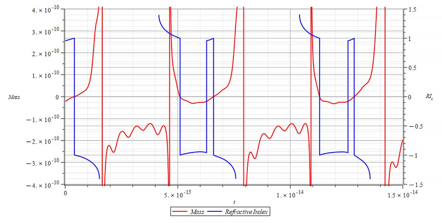
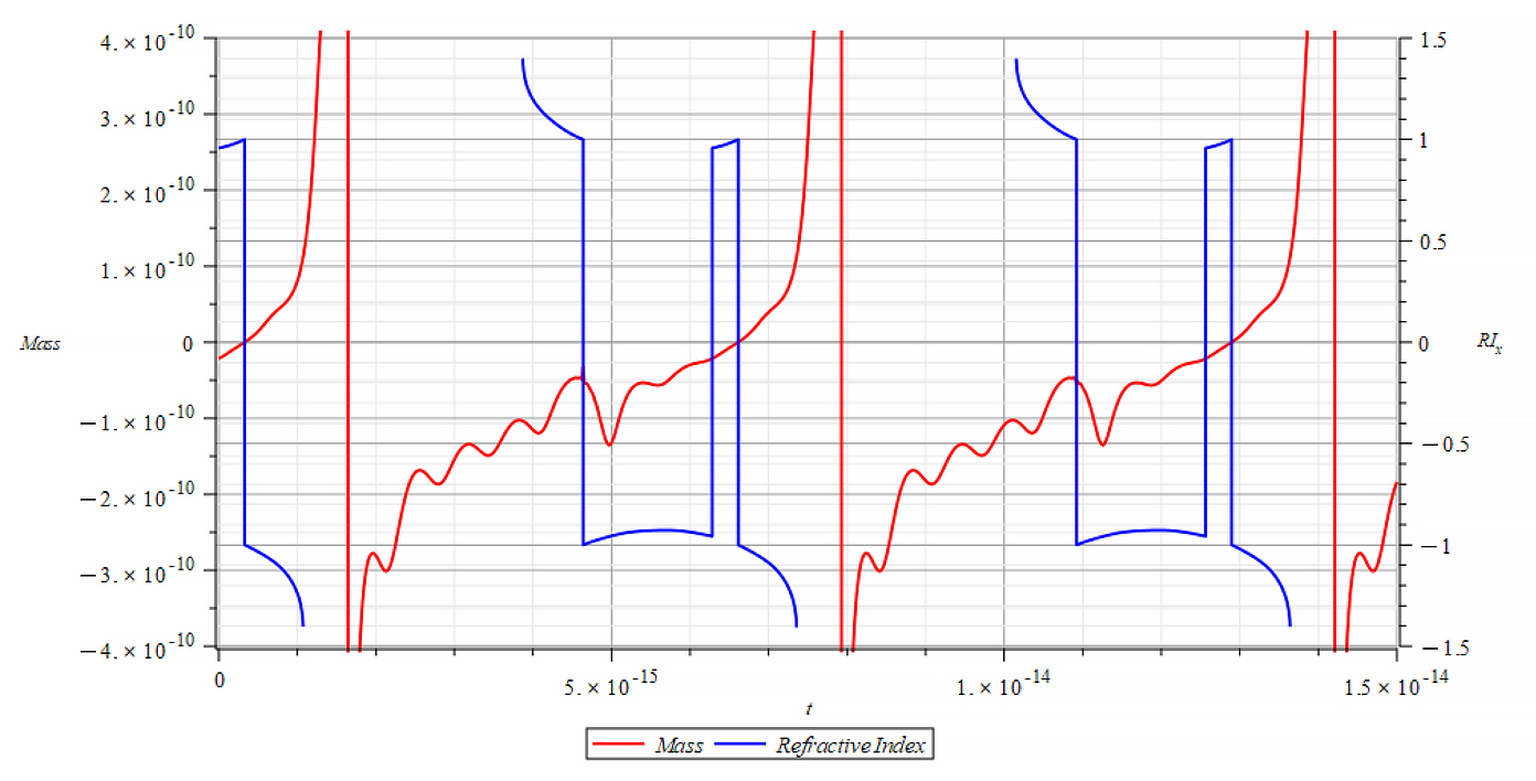
| K=\frac{\omega}{c} Mass & Refractive Index vs. time for the following parameters: \omega=6\ {10}^{14}\ [\frac{1}{s}]; E_m={10}^{24}\ [\frac{V}{m}]; E_f=-1.5\ {10}^{26}\ [\frac{V}{m}] | K=\frac{\omega}{v_{ep}\left(t\right)} Mass & Refractive Index vs. time for the following parameters: \omega=6\ {10}^{14}\ [\frac{1}{s}]; E_m={10}^{24}\ [\frac{V}{m}]; E_f=-1.5\ {10}^{26}\ [\frac{V}{m}] |
For +Ef
 |  |
| K=\frac{\omega}{c} Mass & Refractive Index vs. time for the following parameters: \omega=2\ {10}^{16}\ [\frac{1}{s}]; E_m=8\ {10}^{25}\ [\frac{V}{m}]; E_f={3\ 10}^{26}\ [\frac{V}{m}] | K=\frac{\omega}{v_{ep}\left(t\right)} Mass & Refractive Index vs. time for the following parameters: \omega=2\ {10}^{16}\ [\frac{1}{s}]; E_m=8\ {10}^{25}\ [\frac{V}{m}]; E_f={3\ 10}^{26}\ [\frac{V}{m}] |
For -Ef
 |  |
| K=\frac{\omega}{c} Mass & Refractive Index vs. time for the following parameters: \omega=2\ {10}^{16}\ [\frac{1}{s}]; E_m={10}^{24}\ [\frac{V}{m}]; E_f={-10}^{25}\ [\frac{V}{m}] | K=\frac{\omega}{v_{ep}\left(t\right)} Mass & Refractive Index vs. time for the following parameters: \omega=2\ {10}^{16}\ [\frac{1}{s}]; E_m={10}^{24}\ [\frac{V}{m}]; E_f={-10}^{25}\ [\frac{V}{m}] |
For +Ef
 |  |
| K=\frac{\omega}{c} Mass & Refractive Index vs. time for the following parameters: \omega={10}^{18}\ [\frac{1}{s}]; E_m={10}^{23}\ [\frac{V}{m}]; E_f=2.5\ {10}^{24}\ [\frac{V}{m}] | K=\frac{\omega}{v_{ep}\left(t\right)} Mass & Refractive Index vs. time for the following parameters: \omega={10}^{18}\ [\frac{1}{s}]; E_m={10}^{23}\ [\frac{V}{m}]; E_f=2.5\ {10}^{24}\ [\frac{V}{m}] |
For -Ef
 |  |
| K=\frac{\omega}{c} Mass & Refractive Index vs. time for the following parameters: \omega={10}^{18}\ [\frac{1}{s}]; E_m={10}^{23}\ [\frac{V}{m}]; E_f={-7\ 10}^{24}\ [\frac{V}{m}] | K=\frac{\omega}{v_{ep}\left(t\right)} Mass & Refractive Index vs. time for the following parameters: \omega={10}^{18}\ [\frac{1}{s}]; E_m={10}^{23}\ [\frac{V}{m}]; E_f={-7\ 10}^{24}\ [\frac{V}{m}] |
In Fig. 71 right, we observe that, also during a full negative mass regime, the refractive index changes with mass changes. The Refractive Index depends on the slope of the mass plot, that is, the rate of change of mass.
In general, though this is not the rule, for wave velocity “c”, it decreases with negative mass slope, and vice versa, until reaching the m=0 point, where abruptly switches between n=±1. It seems that the Refractive Index is proportional to the derivative of the mass, and the sign of the derivative changes when the mass sign changes, also at mass minima/maxima (slope = 0) as well as at indeterminate points (slope = ∞).
For wave velocity “v_{ep}\left(t\right)”, the Refractive Index oscillates and switches between n=±1 at m=0 and when the slope of the mass =0. It seems that the refractive index depends on the derivative of the mass.
These are important results that tell us that the refractive index behavior is like a “beacon”, signaling the zones of the negative mass regime, as well as mass changes.
n\ \propto\pm\frac{dm}{dt}
Conclusions
It has been demonstrated that the application of the Universal Electrodynamic Force to the new Atomic Model predicts important changes in nuclear mass when an external force caused by a TEM with an added Static Electric Field is acting on the atomic nucleus.
As we have demonstrated in previous papers, mass is an electrodynamic quantity and as such, it can be manipulated at will. It was demonstrated in this paper that one means to achieve mass changes is not only by striking the nucleus with a TEM but also by the addition of a static electric field.
It was clearly seen from the results, that the magnitude and the sign of the mass can be modified by changing the amplitude and/or frequency of the external wave, within a certain range, and by modifying the magnitude and sign of the static electric field.
The somewhat abrupt sign change of the refractive index values during mass sign change was also clearly demonstrated. There is clear evidence that the refractive index is proportional to the rate of change of the mass, i.e., to the derivative of mass with respect to time.
The refractive index can be used as an aid to search for the negative mass region of the nucleus, as well as in any piece of “macro” material. The refractive index is a “beacon” that signals the exact point of mass sign change and its range, and any mass changes in general.
Fourier’s analysis shows in the phase shift graphs many swings of phase between ±π, which clearly indicate resonance states in the nucleus at those frequencies, as well interferences with the external agent.
In previous papers, we described that the main force that keeps the nuclear shell in a very tight packing structure in such a tiny space is the electrostatic force. This is really an enormous force. It means that we also need huge external electromagnetic fields to achieve some nuclear interaction, and this may represent a technical limitation in the present time.
Bibliography
[1]. Shanshan Yao, Xiaoming Zhou and Gengkai Hu, “Experimental study on negative effective mass in a 1D mass–spring system” (2008), New Journal of Physics (2008). https://iopscience.iop.org/article/10.1088/1367-2630/10/4/043020/pdf
[2]. J. P. Wesley, “Inertial Mass of a Charge in a Uniform Electrostatic Potential Field” (2001), Annales Foundation Louis de Broglie, Volume 26, nr. 4 (2001).
[3]. V. F. Mikhailov, “Influence of an electrostatic potential on the inertial electron mass” (2001), Annales Foundation Louis de Broglie, Volume 26, nr. 4 (2001).
[4]. M. Weikert and M. Tajmar, “Investigation of the Influence of a field-free electrostatic Potential on the Electron Mass with Barkhausen-Kurz Oscillation” (2019), ), Annales Foundation Louis de Broglie, Volume 44, (2019).
[5]. Timothy H. Boyer, “Electrostatic potential energy leading to a gravitational mass change for a system of two point charges” (1979), American Journal of Physics 47, 129 (1979), https://aapt.scitation.org/doi/10.1119/1.11881
[6]. A. K. T. Assis, “Changing the Inertial Mass of a Charged Particle” (1992), Journal of the Physical Society of Japan Vol. 62, No. 5, May, 1993, pp. 1418-142, https://journals.jps.jp/doi/abs/10.1143/JPSJ.62.1418?journalCode=jpsj
[7]. M. Tajmar, “Propellantless propulsion with negative matter generated by electric charges” (2013), Technische Universität Dresden (2013), https://tu-dresden.de/ing/maschinenwesen/ilr/rfs/ressourcen/dateien/forschung/folder-2007-08-21-5231434330/ag_raumfahrtantriebe/JPC—Propellantless-Propulsion-with-Negative-Matter-Generated-by-Electric-Charges.pdf?lang=en
[8]. M. Tajmar and A. K. T. Assis, “Particles with Negative Mass: Production, Properties and Applications for Nuclear Fusion and Self-Acceleration” (2015), https://www.ifi.unicamp.br/~assis/J-Advanced-Phys-V4-p77-82(2015).pdf
[9]. M. A. Khamehchi, Khalid Hossain, M. E. Mossman, Yongping Zhang, Th. Busch, Michael McNeil Forbes, and P. Engels, “Negative-Mass Hydrodynamics in a Spin-Orbit–Coupled Bose-Einstein Condensate” (2017), Phys. Rev. Lett. 118, 155301 (2017), https://journals.aps.org/prl/abstract/10.1103/PhysRevLett.118.155301
[10]. David L. Bergman, J. Paul Wesley, “Spinning Charged Ring Model of Electron Yielding Anomalous Magnetic Moment” (1990).
[11]. Joseph Lucas and Charles W. Lucas, Jr., “A Physical Model for Atoms and Nuclei”, Galilean Electrodynamics, Volume 7, Number 1 (1996), Foundations of Science (2002-2003), Part 1, Part 2, Part 3, Part 4.
[12]. Charles W. Lucas, Jr., “Derivation of the Universal Force Law”, Foundations of Science (2006-2007), Part 1, Part 2, Part 3, Part 4.
[13]. Arthur H. Compton, “The size and shape of the electron” (1918), Journal of the Washington Academy of Sciences, Vol. 8, No. 1, https://www.jstor.org/stable/24521544
[14]. David L. Bergman, “Modeling the Real Structure of an Electron” (2010), Foundations of Science.
[15]. David L. Bergman, “Shape & Size of Electron, Proton & Neutron” (2004), Foundations of Science.
[16]. Zoran Jaksic, N. Dalarsson, Milan Maksimovic, “Negative Refractive Index Metamaterials: Principles and Applications” (2006), https://www.researchgate.net/publication/200162674_Negative_Refractive_Index_Metamaterials_Principles_and_Applications
Related articles:
Negative Mass and Negative Refractive Index in Atom Nuclei – Nuclear Wave Equation – Gravitational and Inertial Control <Part-1>
Negative Mass and Negative Refractive Index in Atom Nuclei – Nuclear Wave Equation – Gravitational and Inertial Control <Part-5>
What is Charge? – The Redefinition of Atom – Energy to Matter Conversion
Nuclear Fusion Enhanced by Negative Mass – A Proposed Method and Device – (Part 1)
Charge Radiation Derived from the Universal Electrodynamic Force – Proof of the Cherenkov Effect
Faster-Than-Light Travel Feasible with Negative Mass – Superluminal Dynamics
New Atomic Model with Real-Valued Wave Function – Energy Levels, Spectrum, and Atomic Fine Structure