
Raul Fattore
April 7, 2023
The present study is divided into six parts
Part-1 Part-2 Part-3 Part-4 Part-5
Table of Contents
In This Paper
This study summarizes the analysis made from Part-1 to Part-5, with a focus on the means we may use to get gravitational and inertial control of mass, as well as some technical constraints based on our present-time technologies.
Abstract
Some efforts have been made to prove negative mass behavior through some experiments performed in mechanics [1], and other disciplines [9], as well as some theories in electrostatics [2,3,4,5,6,7,8], but I haven’t found research about similar effects at the atomic level, where the most elementary mass given by the atomic nucleus is to be found.
- Is the second Newton’s law still valid with negative mass?
- What could happen if we make the atom behave in a negative mass regime?
- Is the negative refractive index related to negative mass?
- Are we able to control the magnitude of mass?
- Are we able to control the sign of mass?
The answers to these questions are given through this series of papers, with results that are coincident with experimental data, except for the negative mass regime. Experiments must be done to confirm or invalidate the theory developed in these articles. Needless to say, if experiments validate this theory, then a significant change in mankind is going to happen. In that case, I strongly ask scientists to cooperate by making use of the derived technologies for good and refrain from doing it for evil.
Introduction
The theory presented in these papers, as described in Part-1, is based on three fundamental aspects that have proved to be extremely effective to describe physical phenomena and predicting results that agree with experimental data [10, 11, 12]:
• Spinning Ring Model of Elementary Particles (toroidal ring of continuous charge)
• New Atomic Model
• The Universal Electrodynamic Force
Based on the new atomic model, a shell arrangement of the nuclear particles has been assumed in Part 1, as shown in Fig. 1.
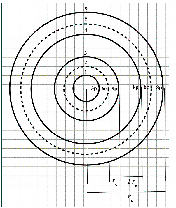
Assumed shell arrangement for Aluminum atomic nucleus
This sandwich configuration keeps the particles very tightly bound together. Note that at three shells in from the outermost shell, there are always two proton shells in a row for the larger nuclides.
This weak binding allows the outermost sandwich of shells to have liquid-like properties and forms the proper justification for a Liquid Drop Model of the nucleus.
As we already know, the torus ring model of the particles has an associated electric field as well as a magnetic field. However, due to the very tight packing configuration of the particles, we may safely assume that the distance among shells is extremely tiny and that the predominant force in the nucleus is of electrostatic origin, while the weaker magnetic forces will add some contribution to the equilibrium distance between each shell. As demonstrated in Part 1, mass is an intrinsic property of the atomic nucleus. Under natural circumstances, it has a constant universal magnitude and is always positive. However, with some proper external agents, we might be able to manipulate the intrinsic mass by changing its magnitude and sign.
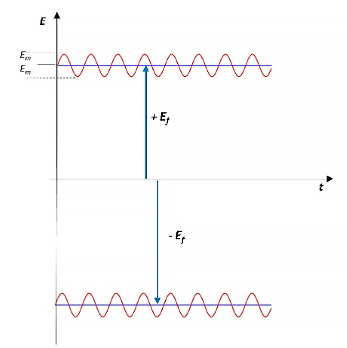
How to make mass changes?
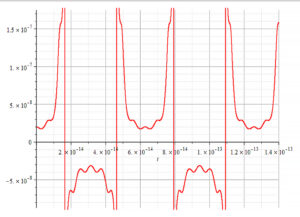
Graph showing negative mass during half periods
We have stated in Part-1 that mass is not a fundamental quantity and demonstrated that depends on the electrodynamics of the atomic nucleus.
More precisely, it depends on the amplitude and frequency of oscillation of the proton and electron shells, which are tightly packed in the nucleus.
As such, we may expect those nuclear shells to react in some way under the action of external forces of electrostatic and/or electrodynamic origin. The reactions of the nuclear shells have been demonstrated in the previous papers, where it was shown there are ways to change not only the mass magnitude but also its sign.
In Fig. 2 we see an example of the oscillatory behavior of mass for natural shells’ self-oscillations, i.e., without applying any external forces. We clearly see the negative mass hemicycles, which most probably average with the positive hemicycles to give the “standard” magnitude of mass under natural conditions.
Throughout this series of papers, it has been uncovered a remarkable property of the oscillatory behavior of the nuclear shells: the main frequency value is the same value of the elementary charge multiplied by some power of ten. This fact might tell us that the fundamental property of matter is not its mass, but rather the elementary charge.
Some methods to change the mass magnitude and sign have been proposed in previous papers, and the nuclear response was analyzed with promising results.
Can We Do Inertial Control?
Inertia can be described as a property of mass due to motion (including the state of “rest”), and it is given by the second law of Newton \vec{F}=m\ \vec{a}. Here the mass is always positive, and the acceleration has the same direction as the acting force. However, if we change the sign and the magnitude of the mass, this equation gives us three situations:
- m > 0: the mass will accelerate in the direction of the force.
- m = 0: if it was previously at “rest”, no matter how big the force could be, the mass will remain at “rest”; if it was previously moving, it will suddenly acquire the “rest” state.
- m < 0: the mass will accelerate in the opposite direction of the force.
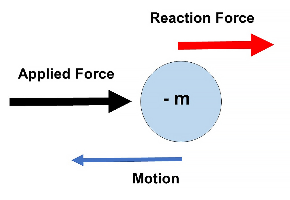
Negative mass response to a force
If we change the magnitude of the mass, the required force to affect the state of motion will also change. Assuming we could reduce the mass of a car to 1 Kg, then we could easily move it. If we make its mass = 0, it will stay still, because no forces will affect it.
If we make its mass <0 and push it, it will “resist” with the same force in the same direction, and when it starts moving, it will do it in our direction. If we pull it, it will run away.
As displayed in Fig. 2a, the reaction force points in the same direction as the applied force. Then, the force needed to start the motion is less than that required when the mass is positive. Friction effects can be masked out with negative mass.
Inertial and Gravitational control working together
By making the magnitude of the mass as small as possible, inertial effects will disappear. The linear momentum will vanish. So will do the centrifugal force and the angular momentum in rotational systems.
The number of applications of inertial control is simply unlimited.
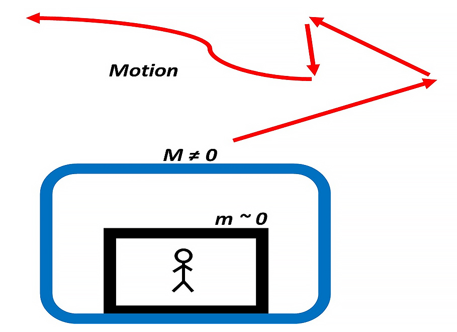
Imagine a vehicle or ship with controlled mass M, of any sign and magnitude different from zero (Fig. 2a.1). A passenger is transported in a cabin of mass m of magnitude near zero.
By controlling the magnitude and sign of mass M, it is possible to achieve huge accelerations or decelerations almost instantly and change motion directions which will defy classic physics because of the inertial effects. However, if we keep the mass m of the passenger cabin near zero, he or she will not feel any inertial discomfort, despite the type of motion.
Are Newton’s laws valid under these conditions? Yes, with one exception. In a negative mass regime, we must change the sign in Newton’s third law. The reaction force points in the same direction as the acting force.
Mathematically, it’s not a violation of Newton’s third law.
Can We Do Gravitational Control?
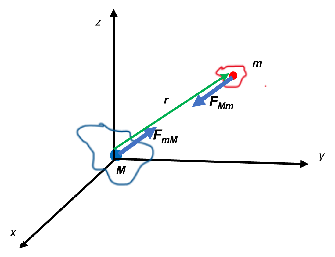
Gravitational forces between two positive masses
Newton’s law of universal gravitation clearly defines the interaction force between two masses as being always attractive. This force is expressed as:
{\vec{F}}_{mM}=-{\vec{F}}_{Mm}=G\ \frac{M\ m}{r^2}\ \hat{r} (a)
The force can be expressed as the relative force seen from any one of the masses:
\vec{F}=-\ G\ \frac{M\ m}{r^2}\ \hat{r} (b)
Looking at Fig. 2b, if both masses are positive, we have that the acceleration induced by M on m is given by: {\vec{a}}_{Mm}=\ G\ \frac{M}{r^2}(-\ \hat{r})=-G\ \frac{M}{r^2}\hat{r}, while the acceleration induced by m on M is given by: {\vec{a}}_{mM}=G\ \frac{m}{r^2}\ \hat{r}.
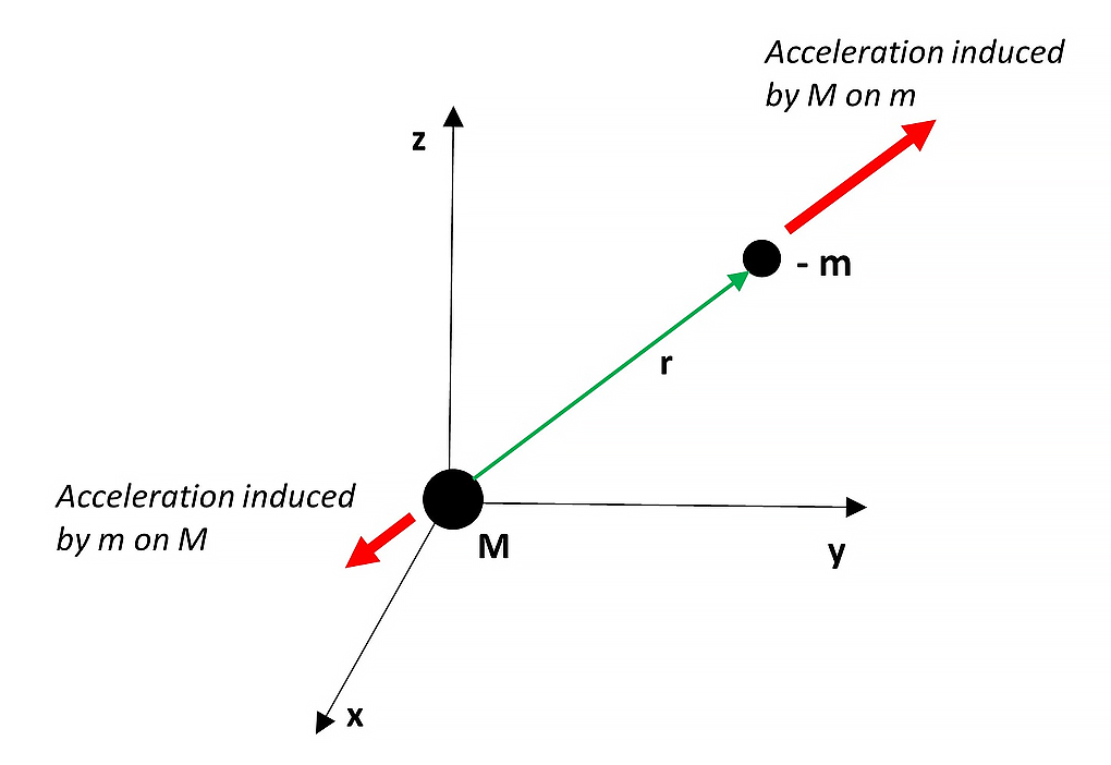
Gravitational forces between positive and negative mass
Assume now the mass m is negative, i.e., -m. Based on Fig. 2a, now the acceleration induced by M on m will point in the opposite direction {\vec{a}}_{Mm}=\ G\ \frac{M}{r^2}(+\ \hat{r}). On the other hand, the acceleration induced now by -m on M is given by: {\vec{a}}_{mM}=G\ \frac{(-m)}{r^2}\ \hat{r}=-\ G\ \frac{m}{r^2}\ \hat{r}.
We clearly see that the accelerations on each mass point in opposite directions, as shown in Fig. 2c.
We can confirm the results above by applying Newton’s second law on every mass in Eq. (b). The acceleration of mass M induced by -m is: M\ a_M\hat{r}=-\ G\ \frac{M\ (-m)}{r^2}\ \hat{r}, that is a_M=G\ \frac{m}{r^2}. On the other hand, and considering second Newton’s law for negative mass, the acceleration of mass -m induced by M is: (-m)(-\ a_m)\hat{r}=-\ G\ \frac{M\ (-m)}{r^2}\ \hat{r}, that is a_m=G\ \frac{M}{r^2}.
So, once more, we see that the acceleration on each mass is positive, which is a clear repulsion condition.
The easiest way to see this effect is by simply applying Newton’s gravitational law given by Eq. (b). The relative force seen by any one of the masses becomes:
\vec{F}=-\ G\ \frac{M\ (-m)}{r^2}\ \hat{r}\ =G\ \frac{M\ m}{r^2}\ \hat{r} (c)
This is clearly a repulsive force.
If M>>m, the acceleration on m will have a considerable magnitude, while mass M will not perceive any effects.
It has been demonstrated in this series of papers that the mass sign and magnitude can be modified at will. Therefore, Gravitational Control can be achieved.
Proposed Methods to Change Mass Magnitude and Sign
The Aluminum atom was chosen for this study, and the results obtained throughout all papers are based on the nuclear structure as shown in Fig. 1. Why Aluminum? Because is an easy material to find, which is used in many objects and vehicles, and could be easily used in experiments to check the results published in this series of papers.
The suggested methods for mass modification are basically very simple but involve technical constraints based on the levels of energy needed to obtain a nuclear response.
Basically, the three methods proposed consist of applying external forces to the nucleus based on electrostatic and electrodynamic fields:
- Transverse Polarized Electromagnetic Wave (TEM)
- Transverse Polarized Electromagnetic Wave (TEM) plus Static Electric Field
- Electric Signal plus Static Electric Field
1. Mass Control with a Transverse Polarized Electromagnetic Wave (TEM)
The effects on the nucleus caused by the force originated by a TEM have been dealt with in detail in Part-3. It was demonstrated how to change the mass magnitude and sign by changing the amplitude or frequency of the wave.
Contour or level graph of mass
To have a more approximate idea of the values of amplitude and frequency required to obtain the mass magnitude and sign changes, the mass was averaged to make it independent of time, and its magnitude has been plotted as level lines (or contour lines) as a function of the wave amplitude and frequency.
Fig. 3 shows how to understand the graph of wave amplitude as a function of frequency. The thick blue line delimits the region of positive mass, while the thick red line delimits the region of negative mass.
The following graphs display some examples of mass magnitude and sign with respect to wave amplitude and frequency.
1a. Results for Wave Velocity v ≠ “c” in the nucleus (partial or total energy absorption)
The external force was integrated for the travel time of the wave in the nucleus, with velocity v ≠ c, as given by Eq. (4) in Part-3.
The main parameters used for the mass calculations are:
r_n=3.5\ {10}^{-15}\ [m]; A_e=2\ {10}^{-16}\ [m]; A_p={10}^{-3}A_e\ [m]; N_0=378; N_s=312
\omega_e={10}^{15}\ [\frac{1}{s}]; \omega_p={10}^{16}\ [\frac{1}{s}]
Contour graph of mass for wave parameters range:
\omega=0\ to\ 5\ {10}^{14}\ [\frac{1}{s}] – E_m=0\ to\ 5\ {10}^{14}\ [\frac{V}{m}]
In Fig. 4 we see the thick blue lines delimiting/enclosing the regions of positive mass, while the thick red line, which is in the upper-left side of the graph, delimits the negative mass region.
In this case, the frequency range for negative mass control is limited to a band in the lower frequencies, with high amplitudes.
However, for positive mass control, there are several frequency bands of choice, with a wider range of amplitude.
Contour graph of mass for wave parameters range:
\omega=0\ to\ {10}^{13}\ [\frac{1}{s}] – E_m=0\ to\ {10}^{17}\ [\frac{V}{m}]
Fig. 5 is displaying quite the opposite of the situation in Fig. 4.
The delimiting lines of mass sign run almost parallel to the vertical axis for the lower frequencies, by having a wide range of amplitudes. In this region, mass sign change using frequency could be sensitive to little frequency changes. These regions of alternating mass sign repeat to the right for higher frequencies until we observe only regions of negative mass on the right.
Contour graph of mass for wave parameters range:
\omega=0\ to\ {10}^{15}\ [\frac{1}{s}] – E_m=0\ to\ {10}^{15}\ [\frac{V}{m}]
Fig. 6 displays a similar situation to that in Fig. 5.
We clearly see the wide alternating regions of positive and negative mass.
A good aspect here is that the regions are wider than those in Fig. 4 and Fig. 5, allowing thus to control the mass magnitude and sign within a wider range of frequency.
In this case, we must consider the fact that the amplitude increases approximately linearly with the selected work frequency.
1b. Results for Wave Velocity v ≠ “c” in the nucleus (partial or total energy absorption)
The external force was integrated over a wave period, with velocity v ≠ c, as given by Eq. (6) in Part-3.
The main parameters used for the mass calculations are:
r_n=3.5\ {10}^{-15}\ [m]; A_e=2\ {10}^{-16}\ [m]; A_p={10}^{-3}A_e\ [m]; N_0=378; N_s=312
\omega_e={10}^{15}\ [\frac{1}{s}]; \omega_p={10}^{16}\ [\frac{1}{s}]
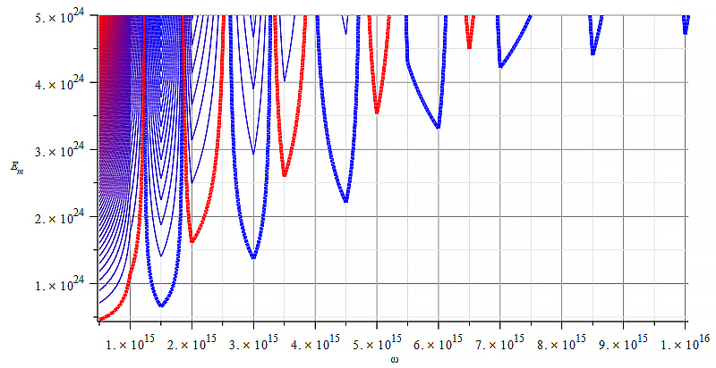 |  |
| Figure 7 Contour graph of mass for wave parameters range: \omega=0\ to\ 5\ {10}^{16}\ [\frac{1}{s}]; E_m=0\ to\ 5\ {10}^{24}\ [\frac{V}{m}] | Figure 8 Contour graph of mass for wave parameters range: \omega=0\ to\ {10}^{10}\ [\frac{1}{s}]; E_m=0\ to\ 3\ {10}^{18}\ [\frac{V}{m}] |
Contour graph of mass for wave parameters range:
\omega=0\ to\ {10}^{12}\ [\frac{1}{s}]; E_m=0\ to\ {5\ 10}^{17}\ [\frac{V}{m}]
The method of integration of the force over a wave period, for wave velocity v ≠ “c”, yields results somewhat like those shown in paragraph 1a.
In comparison, the values of wave amplitudes for mass control are higher here, while wave frequencies are lower.
We see in Fig.7 that the amplitude increases approximately linearly with the selected work frequency.
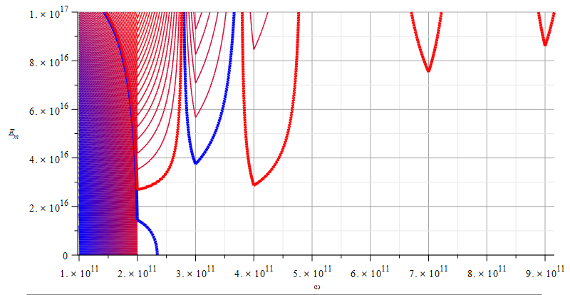
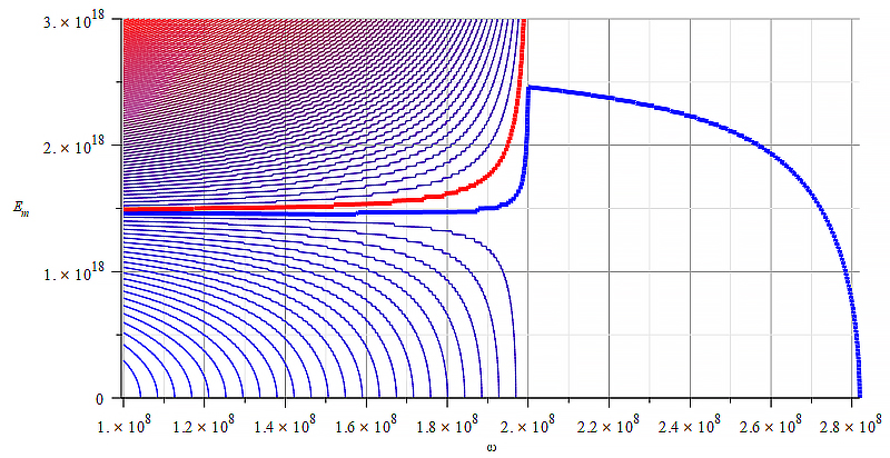
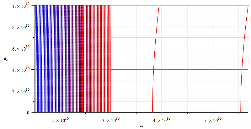
1c. Results for Wave Velocity v = “c” in the nucleus (energy transmission)
The external force was integrated for the travel time of the wave in the nucleus, with velocity v = c, as given by Eq. (5) in Part-3.
The main parameters used for the mass calculations are:
r_n=3.5\ {10}^{-15}\ [m]; A_e=2\ {10}^{-16}\ [m]; A_p={10}^{-3}A_e\ [m]; N_0=378; N_s=312
\omega_e={10}^{15}\ [\frac{1}{s}]; \omega_p={10}^{16}\ [\frac{1}{s}]
 | 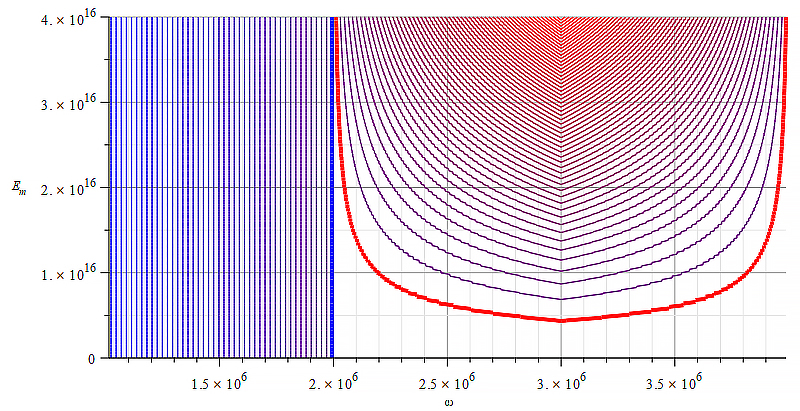 |
| Figure 10 Contour graph of mass for wave parameters range: \omega=0\ to\ {10}^{11}\ [\frac{1}{s}]; E_m=0\ to\ 7\ {10}^{14}\ [\frac{V}{m}] | Figure 11 Contour graph of mass for wave parameters range: \omega=0\ to\ {10}^8\ [\frac{1}{s}]; E_m=0\ to\ 4\ {10}^{16}\ [\frac{V}{m}] |
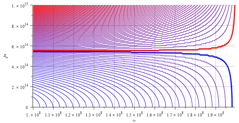
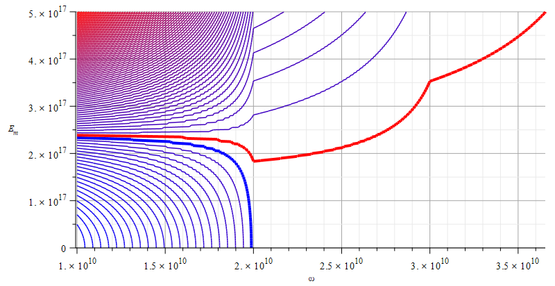
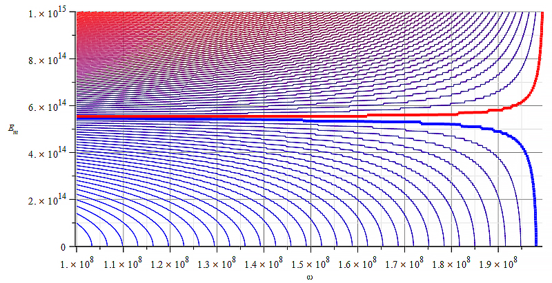
Contour graph of mass for wave parameters range:
\omega=0\ to\ {10}^{10}\ [\frac{1}{s}]; E_m=0\ to\ {10}^{15}\ [\frac{V}{m}]
In Fig. 10 we may use the wave amplitude to easily change the mass sign while varying the wave frequency to get different mass magnitudes within the chosen range.
In Fig. 11, the change of mass sign is easier done by varying the wave frequency (for a certain minimum amplitude). Within the negative mass zone, we may change the mass magnitude, whether with the wave amplitude or frequency.
However, within the positive mass zone, the mass magnitude can only be modified with the wave frequency. In Fig. 12 we observe similar behavior as seen in Fig. 10.
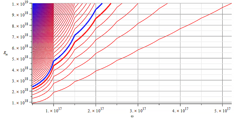
1d. Results for Wave Velocity v = “c” in the nucleus (partial or total energy absorption)
The external force was integrated over a wave period, with velocity v = c, as given by Eq. (6) in Part-3.
The main parameters used for the mass calculations are:
r_n=3.5\ {10}^{-15}\ [m]; A_e=2\ {10}^{-16}\ [m]; A_p={10}^{-3}A_e\ [m]; N_0=378; N_s=312
\omega_e={10}^{15}\ [\frac{1}{s}]; \omega_p={10}^{16}\ [\frac{1}{s}]
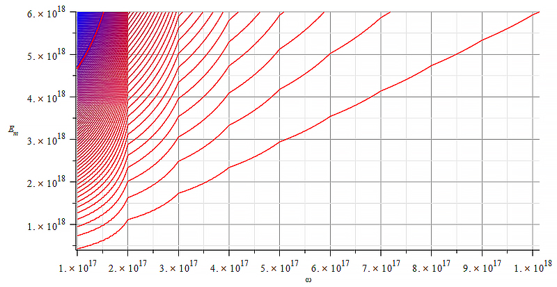 |  |
| Figure 13 Contour graph of mass for wave parameters range: \omega=0\ to\ {10}^{19}\ [\frac{1}{s}]; E_m=0\ to\ 6\ {10}^{18}\ [\frac{V}{m}] | Figure 14 Contour graph of mass for wave parameters range: \omega=0\ to\ {1.5\ 10}^{18}\ [\frac{1}{s}]; E_m=0\ to\ {10}^{17}\ [\frac{V}{m}] |
In Fig. 13, the separation of positive and negative mass zones is located on the upper-left side of the graph, making the mass control very sensitive to both: wave amplitude and frequency.
Contour graph of mass for wave parameters range:
\omega=0\ to\ {5\ 10}^{18}\ [\frac{1}{s}]; E_m=0\ to\ {10}^{19}\ [\frac{V}{m}]
In Fig. 14 we see that the mass sign and magnitude can be easily controlled by the wave frequency, at any amplitude value within the range.
In Fig. 15, we observe a quasi-linear relationship between wave amplitude and frequency, allowing thus smooth mass control. As demonstrated in the examples given in the previous figures, mass magnitude, and sign control could be possible by applying an external force on the nucleus caused by a Transverse Polarized Electromagnetic Wave.
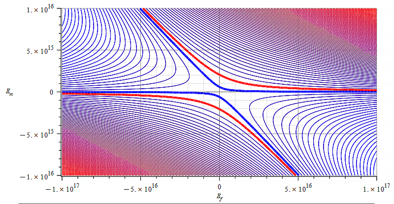
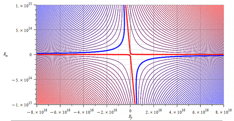
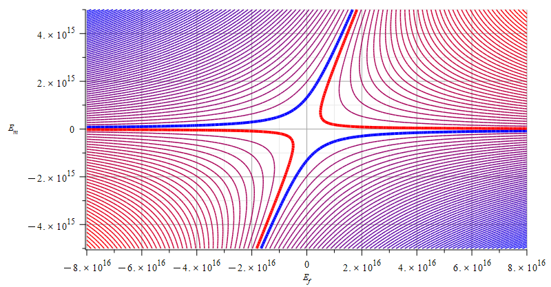
2. Mass Control with a Transverse Polarized Electromagnetic Wave (TEM) plus a Static Electric Field
The effects on the nucleus caused by the force originated by a TEM plus a static electric field have been dealt with in detail in Part-3. It was demonstrated how to change the mass magnitude and sign by changing the amplitude or frequency of the wave, as well as the magnitude and polarity of the static electric field.
2a. Results for Wave Velocity v ≠ “c” in the nucleus (partial or total energy absorption)
The external force was integrated for the travel time of the wave in the nucleus, with velocity v ≠ c, as given by Eq. (4) in Part-3.
The main parameters used for the mass calculations are:
r_n=3.5\ {10}^{-15}\ [m]; A_e=2\ {10}^{-16}\ [m]; A_p={10}^{-3}A_e\ [m]; N_0=378; N_s=312
\omega_e={10}^{15}\ [\frac{1}{s}]; \omega_p={10}^{16}\ [\frac{1}{s}]
 |  |
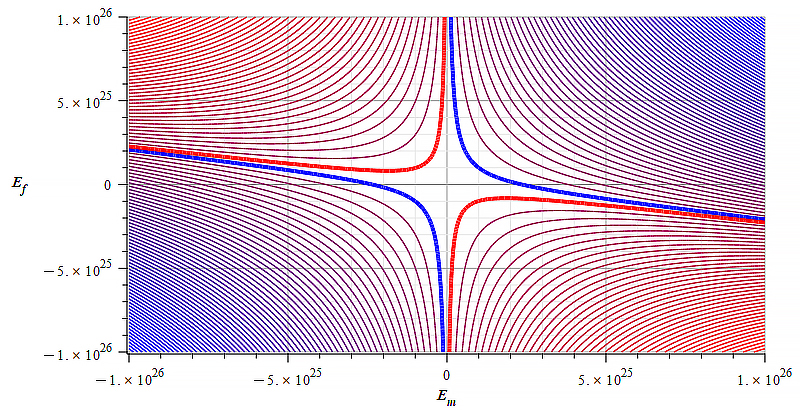
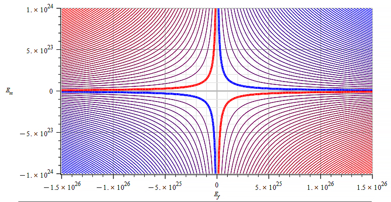
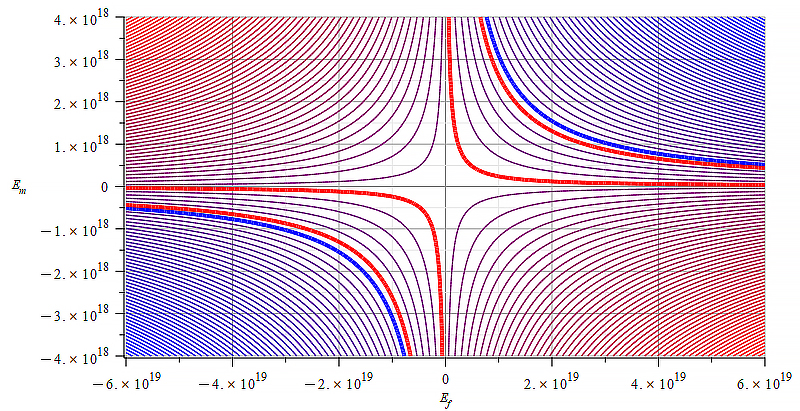
| Figure 16 Contour graph of mass for: \omega={10}^{14}\ [\frac{1}{s}]; E_m=-{10}^{23}\ to\ {10}^{23}\ [\frac{V}{m}]; E_f=-{10}^{26}\ to\ {10}^{26}\ [\frac{V}{m}] | Figure 17 Contour graph of mass for: \omega={10}^{14}\ [\frac{1}{s}]; E_m=-{10}^{26}\ to\ {10}^{26}\ [\frac{V}{m}]; E_f=-{3\ 10}^{25}\ to\ {3\ 10}^{25}\ [\frac{V}{m}] |
 |  |
| Figure 18 Contour graph of mass for: \omega={10}^{12}\ [\frac{1}{s}]; E_m=-{10}^{26}\ to\ {10}^{26}\ [\frac{V}{m}]; E_f=-{10}^{26}\ to\ {10}^{26}\ [\frac{V}{m}] | Figure 19 Contour graph of mass for: \omega={10}^{12}\ [\frac{1}{s}]; E_m=-{10}^{26}\ to\ {10}^{26}\ [\frac{V}{m}]; E_f=-{3\ 10}^{25}\ to\ {3\ 10}^{25}\ [\frac{V}{m}] |
 |  |
| Figure 20 Contour graph of mass for: \omega={10}^{19}\ [\frac{1}{s}]; E_m=-{10}^{23}\ to\ {10}^{23}\ [\frac{V}{m}]; E_f=-{10}^{26}\ to\ {10}^{26}\ [\frac{V}{m}] | Figure 21 Contour graph of mass for: \omega={10}^{19}\ [\frac{1}{s}]; E_m=-{10}^{26}\ to\ {10}^{26}\ [\frac{V}{m}]; E_f=-{10}^{26}\ to\ {10}^{26}\ [\frac{V}{m}] |
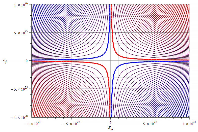
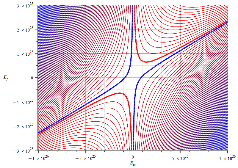
Static electric field added to wave amplitude
The graphs above depict the magnitude and sign of the mass in level curves (contours) with respect to the static electric field amplitude and wave amplitude, for a certain wave frequency.
Observe that the static electric field magnitude is in the vertical axis in Fig. 16 to Fig. 21.
To get mass control, we must consider an adequate relationship between the electric field magnitude and the wave amplitude.
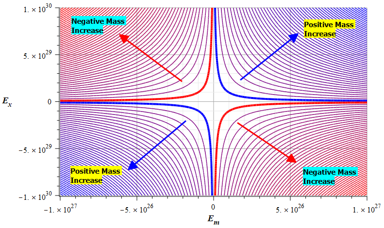
The results displayed in Fig. 16 and Fig. 20 are based on the relationship shown in Fig. 22 (not in scale). Positive mass could never be obtained in such a case for certain wave frequencies.
Results as those displayed in Fig. 17 and Fig. 21 show better conditions for mass sign and magnitude control by changing the wave amplitude, as well as the electric field amplitude and polarity.
2b. Results for Wave Velocity v ≠ “c” in the nucleus (partial or total energy absorption)
The external force was integrated over a wave period, with velocity v ≠ c, as given by Eq. (6) in Part-3.
The main parameters used for the mass calculations are:
r_n=3.5\ {10}^{-15}\ [m]; A_e=2\ {10}^{-16}\ [m]; A_p={10}^{-3}A_e\ [m]; N_0=378; N_s=312
\omega_e={10}^{15}\ [\frac{1}{s}]; \omega_p={10}^{16}\ [\frac{1}{s}]
 |  |
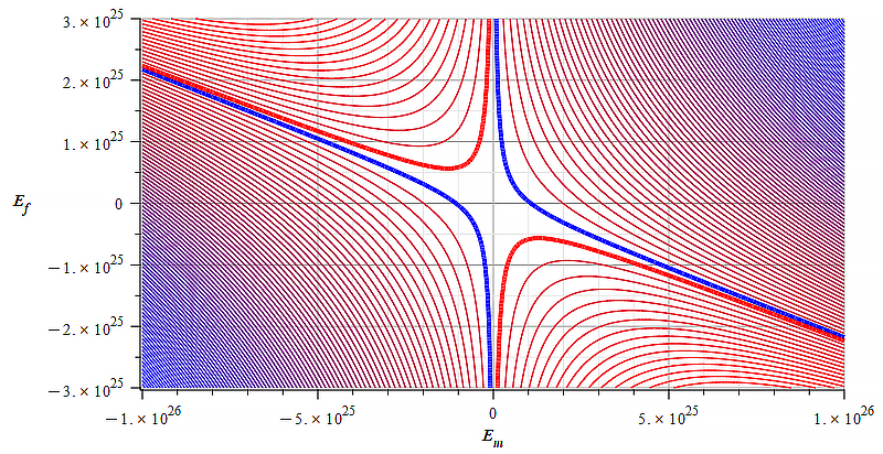
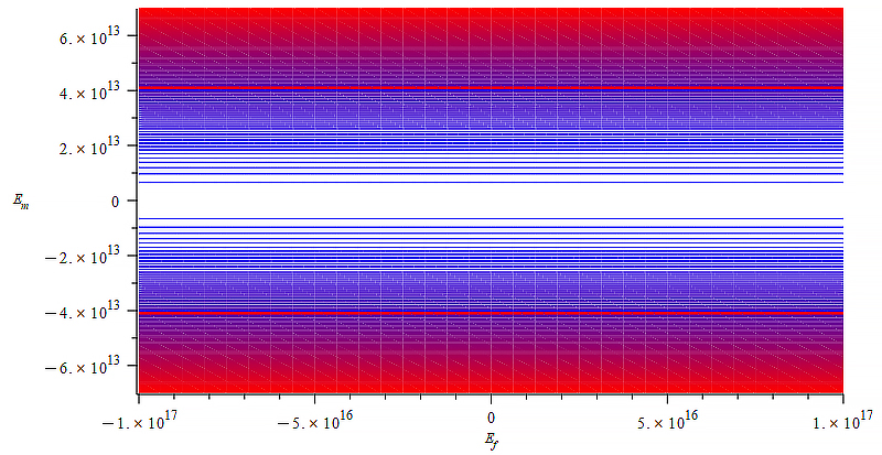
| Figure 23 Contour graph of mass for: \omega={10}^{12}\ [\frac{1}{s}]; E_m=-{10}^{16}\ to\ {10}^{16}\ [\frac{V}{m}]; E_f=-{10}^{17}\ to\ {10}^{17}\ [\frac{V}{m}] | Figure 24 Contour graph of mass for: \omega={10}^{14}\ [\frac{1}{s}]; E_m=-{10}^{15}\ to\ {10}^{15}\ [\frac{V}{m}]; E_f=-{8\ 10}^{16}\ to\ {8\ 10}^{16}\ [\frac{V}{m}] |
Contour graph of mass for:
\omega={10}^{17}\ [\frac{1}{s}]; E_m=-5\ {10}^{15}\ to\ 5\ {10}^{15}\ [\frac{V}{m}]; E_f=-{8\ 10}^{16}\ to\ {8\ 10}^{16}\ [\frac{V}{m}]
Observe that the static electric field magnitude is in the horizontal axis in Fig. 23 to Fig. 25.
As stated in the previous paragraph, it is very important to choose a reasonable relationship between static electric field magnitude and wave amplitude, to allow mass sign and magnitude changes as smoothly as possible.
These figures are not good examples, though decent conditions are those displayed in Fig. 25.
2c. Results for Wave Velocity v = “c” in the nucleus (energy transmission)
The external force was integrated for the travel time of the wave in the nucleus, with velocity v = c, as given by Eq. (5) in Part-3.
The main parameters used for the mass calculations are:
r_n=3.5\ {10}^{-15}\ [m]; A_e=2\ {10}^{-16}\ [m]; A_p={10}^{-3}A_e\ [m]; N_0=378; N_s=312
\omega_e={10}^{15}\ [\frac{1}{s}]; \omega_p={10}^{16}\ [\frac{1}{s}]
 |  |
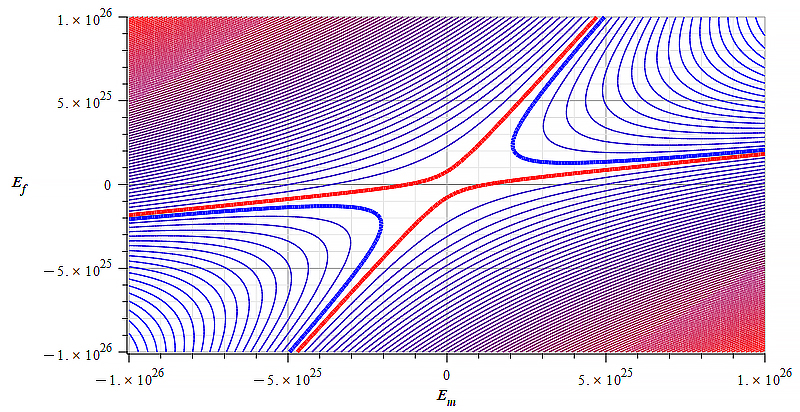
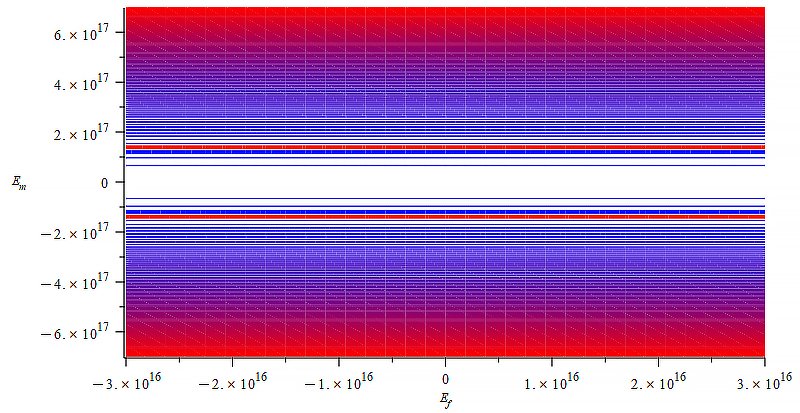
| Figure 26 Contour graph of mass for: \omega=1.6\ {10}^{15}\ [\frac{1}{s}]; E_m=-{10}^{17}\ to\ {10}^{17}\ [\frac{V}{m}]; E_f=-{10}^{18}\ to\ {10}^{18}\ [\frac{V}{m}] | Figure 27 Contour graph of mass for: \omega={10}^8\ [\frac{1}{s}]; E_m=-{7\ 10}^{13}\ to\ 7\ {10}^{13}\ [\frac{V}{m}]; E_f=-{10}^{18}\ to\ {10}^{18}\ [\frac{V}{m}] |
Contour graph of mass for:
\omega={10}^{15}\ [\frac{1}{s}]; E_m=-7\ {10}^{17}\ to\ 7\ {10}^{17}\ [\frac{V}{m}]; E_f=-{3\ 10}^{16}\ to\ {3\ 10}^{16}\ [\frac{V}{m}]
Observe that the static electric field magnitude is now in the horizontal axis in Fig. 26 to Fig. 28, while the vertical axis is the wave amplitude (E_w=E_m).
The only possibility we have to control the mass magnitude and sign is by changing the wave amplitude. For the given conditions, changes in the static electric field magnitude have no effect on mass.
2d. Results for Wave Velocity v = “c” in the nucleus (partial or total energy absorption)
The external force was integrated over a wave period, with velocity v = c, as given by Eq. (6) in Part-3.
The main parameters used for the mass calculations are:
r_n=3.5\ {10}^{-15}\ [m]; A_e=2\ {10}^{-16}\ [m]; A_p={10}^{-3}A_e\ [m]; N_0=378; N_s=312
\omega_e={10}^{15}\ [\frac{1}{s}]; \omega_p={10}^{16}\ [\frac{1}{s}]
 |  |
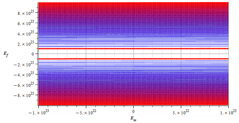
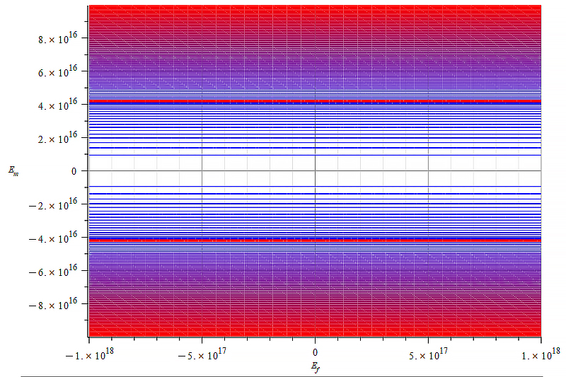
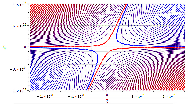
| Figure 29 Contour graph of mass for: \omega=6\ {10}^{14}\ [\frac{1}{s}]; E_m=-{10}^{24}\ to\ {10}^{24}\ [\frac{V}{m}]; E_f=-{1.5\ 10}^{26}\ to\ {1.5\ 10}^{26}\ [\frac{V}{m}] | Figure 30 Contour graph of mass for: \omega={2\ 10}^{16}\ [\frac{1}{s}]; E_m=-{4\ 10}^{18}\ to\ 4\ {10}^{18}\ [\frac{V}{m}]; E_f=-{\ 6\ 10}^{19}\ to\ {\ 6\ 10}^{19}\ [\frac{V}{m}] |
Contour graph of mass for:
\omega={10}^{18}\ [\frac{1}{s}]; E_m=-{10}^{23}\ to\ {10}^{23}\ [\frac{V}{m}]; E_f=-{2.5\ 10}^{24}\ to\ {2.5\ 10}^{24}\ [\frac{V}{m}]
Observe that the static electric field magnitude is in the horizontal axis in Fig. 29 to Fig. 31, while the vertical axis is the wave amplitude (E_w=E_m).
Fig. 29 doesn’t offer good conditions for mass control with any of the external agents.
However, in Fig. 30 and Fig. 31, mass sign and magnitude control can be better achieved within a good range of wave amplitude, for both polarities of the static electric field.
3. Mass Control with an Electric Signal plus a Static Electric Field
The effects on the nucleus caused by the force originated by a TEM plus a static electric field have been dealt with in detail in Part-3. It was demonstrated how to change the mass magnitude and sign by changing the amplitude or frequency of the wave, as well as the magnitude and polarity of the static electric field.
3a. Results obtained of the Force produced by an Electric Signal plus a Static Electric Field on the Nucleus
The external force was integrated over the entire volume of the nucleus and is given by Eq. (4) in Part-5.
The main parameters used for the mass calculations are:
r_n=3.5\ {10}^{-15}\ [m]; A_e=2\ {10}^{-16}\ [m]; A_p={10}^{-3}A_e\ [m]; N_0=378; N_s=312
\omega_e={10}^{15}\ [\frac{1}{s}]; \omega_p={10}^{16}\ [\frac{1}{s}]
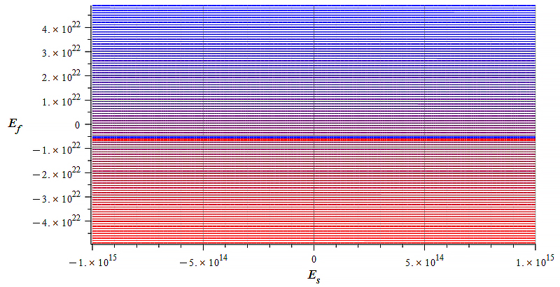 | 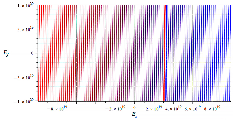 |
| Figure 32 Contour graph of mass for: \omega=2.4\ {10}^{17}\ [\frac{1}{s}]; E_s=-{10}^{15}\ to\ {10}^{15}\ [\frac{V}{m}]; E_f=-{5\ 10}^{22}\ to\ {5\ 10}^{22}\ [\frac{V}{m}] | Figure 33 Contour graph of mass for: \omega={1.3\ 10}^{17}\ [\frac{1}{s}]; E_s=-{10}^{20}\ to\ {10}^{20}\ [\frac{V}{m}]; E_f=-{\ 10}^{20}\ to\ {\ 10}^{20}\ [\frac{V}{m}] |
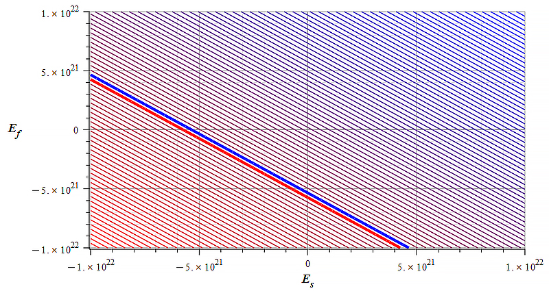
Contour graph of mass for:
\omega={10}^{14}\ [\frac{1}{s}]; E_s=-{10}^{22}\ to\ {10}^{22}\ [\frac{V}{m}]; E_f=-{10}^{22}\ to\ {10}^{22}\ [\frac{V}{m}]
Observe that the static electric field magnitude is in the vertical axis in Fig. 32 to Fig. 34, while the horizontal axis is the signal amplitude.
We see in Fig. 32 that mass sign and magnitude control can be easily done by changing the polarity and magnitude of the static electric field, while signal amplitude has no effect on mass change within the displayed range.
However, mass control in Fig.33 is performed by varying the signal amplitude, while the static electric field has no effect within the given range.
Fig. 34 displays an intermediate situation between Fig. 32 and Fig. 33, where both, signal amplitude and electric field magnitude can be used for mass control.
Technical Limitations and Feasibility
The study developed in this series of papers was based on the nucleus of the Aluminum atom, just to make it as realistic as possible with an easy-to-find material that can eventually be used to perform experiments to check the theory presented here.
Aluminum has an electrical breakdown strength of approximately 15\ {10}^6\ [\frac{V}{m}]. Contemporary known materials and metamaterials with the highest known electrical breakdown strength are insulators, with approximate values of 120\ {10}^6\ [\frac{V}{m}] for Mica, 170\ {10}^6\ [\frac{V}{m}] for Teflon, and 2\ {10}^9\ [\frac{V}{m}] for Diamond.
The nuclear response has been analyzed by applying external agents to the nucleus, such as Transverse Polarized Electromagnetic Wave (TEM), Electric Signal, and Static Electric Field. To obtain some reasonable results, the amplitudes of the wave and signal, as well as the magnitude of the electric field, needed to be set at certain values that are far beyond the electrical breakdown of the Aluminum. Moreover, the set magnitudes are only theoretical values, impossible to be technically achieved.
What is the purpose of the Static Electric Field?
It has been demonstrated that the mass sign and magnitude can be modified at will with an external wave or electric signal, by changing the amplitude and operating frequency. The limitation here is that we don’t have a “steering force”. By additionally applying a static electric field, we make the force have the same direction as the field. So, we may direct the force in the direction we wish.
If we can create a longitudinal polarized wave, then we can dismiss the static electric field.
What To Do?
The very tight nuclear packing structure of the shells requires huge amounts of energy to get some interaction effects. As such, the magnitude of the external fields needs to be extremely high. This is a nuclear property that applies to any material. Therefore, more investigation is required to find some way to overcome these constraints.
Investigating the nuclear response is not an easy task in the laboratory. It might be difficult, time-consuming, and of course, expensive.
The negative effective mass has already been obtained in a simple oscillatory mechanical system [1]. There is no reason to not do the same in electronics, in a relatively short time. But how?
An idea could be to simulate the nuclear structure by making a “macro” nucleus in the form of a multi-layer spherical capacitor. This way, we can manipulate such a capacitor structure to simulate not only existing materials but also “create new ones” that deliver the expected results.
Once we get negative effective mass results with such a capacitor, we can reduce it to the nanoscale and make some sort of metamaterial with controlled properties.
Experiments are needed to validate any theory. And to make things happen.
Conclusions
It has been demonstrated that the application of the Universal Electrodynamic Force to the new Atomic Model predicts important changes in nuclear mass when an external force caused by an Electric Signal with an added Static Electric Field is acting on the atomic nucleus.
As we have demonstrated in previous papers, mass is an electrodynamic quantity and as such, it can be manipulated at will. It was demonstrated in this paper that besides the previously analyzed external agents, one more mean can be used to achieve mass changes.
It has been demonstrated that the magnitude and the sign of the mass can be modified by changing the amplitude and/or frequency of an external wave or signal, within a certain range, as well as by modifying the magnitude and sign of an external static electric field.
In previous papers, we described that the main force that keeps the nuclear shell in a very tight packing structure in such a tiny space is the electrostatic force. This is really an enormous force. It means that we also need huge external electromagnetic fields to achieve some nuclear interaction, and this may represent a technical limitation in the present time.
Bibliography
[1]. Shanshan Yao, Xiaoming Zhou and Gengkai Hu, “Experimental study on negative effective mass in a 1D mass–spring system” (2008), New Journal of Physics (2008). https://iopscience.iop.org/article/10.1088/1367-2630/10/4/043020/pdf
[2]. J. P. Wesley, “Inertial Mass of a Charge in a Uniform Electrostatic Potential Field” (2001), Annales Foundation Louis de Broglie, Volume 26, nr. 4 (2001).
[3]. V. F. Mikhailov, “Influence of an electrostatic potential on the inertial electron mass” (2001), Annales Foundation Louis de Broglie, Volume 26, nr. 4 (2001).
[4]. M. Weikert and M. Tajmar, “Investigation of the Influence of a field-free electrostatic Potential on the Electron Mass with Barkhausen-Kurz Oscillation” (2019), ), Annales Foundation Louis de Broglie, Volume 44, (2019).
[5]. Timothy H. Boyer, “Electrostatic potential energy leading to a gravitational mass change for a system of two point charges” (1979), American Journal of Physics 47, 129 (1979), https://aapt.scitation.org/doi/10.1119/1.11881
[6]. A. K. T. Assis, “Changing the Inertial Mass of a Charged Particle” (1992), Journal of the Physical Society of Japan Vol. 62, No. 5, May, 1993, pp. 1418-142, https://journals.jps.jp/doi/abs/10.1143/JPSJ.62.1418?journalCode=jpsj
[7]. M. Tajmar, “Propellantless propulsion with negative matter generated by electric charges” (2013), Technische Universität Dresden (2013), https://tu-dresden.de/ing/maschinenwesen/ilr/rfs/ressourcen/dateien/forschung/folder-2007-08-21-5231434330/ag_raumfahrtantriebe/JPC—Propellantless-Propulsion-with-Negative-Matter-Generated-by-Electric-Charges.pdf?lang=en
[8]. M. Tajmar and A. K. T. Assis, “Particles with Negative Mass: Production, Properties and Applications for Nuclear Fusion and Self-Acceleration” (2015), https://www.ifi.unicamp.br/~assis/J-Advanced-Phys-V4-p77-82(2015).pdf
[9]. M. A. Khamehchi, Khalid Hossain, M. E. Mossman, Yongping Zhang, Th. Busch, Michael McNeil Forbes, and P. Engels, “Negative-Mass Hydrodynamics in a Spin-Orbit–Coupled Bose-Einstein Condensate” (2017), Phys. Rev. Lett. 118, 155301 (2017), https://journals.aps.org/prl/abstract/10.1103/PhysRevLett.118.155301
[10]. David L. Bergman, J. Paul Wesley, “Spinning Charged Ring Model of Electron Yielding Anomalous Magnetic Moment” (1990).
[11]. Joseph Lucas and Charles W. Lucas, Jr., “A Physical Model for Atoms and Nuclei”, Galilean Electrodynamics, Volume 7, Number 1 (1996), Foundations of Science (2002-2003), Part 1, Part 2, Part 3, Part 4.
[12]. Charles W. Lucas, Jr., “Derivation of the Universal Force Law”, Foundations of Science (2006-2007), Part 1, Part 2, Part 3, Part 4.
[13]. Arthur H. Compton, “The size and shape of the electron” (1918), Journal of the Washington Academy of Sciences, Vol. 8, No. 1, https://www.jstor.org/stable/24521544
[14]. David L. Bergman, “Modeling the Real Structure of an Electron” (2010), Foundations of Science.
[15]. David L. Bergman, “Shape & Size of Electron, Proton & Neutron” (2004), Foundations of Science.
[16]. Zoran Jaksic, N. Dalarsson, Milan Maksimovic, “Negative Refractive Index Metamaterials: Principles and Applications” (2006), https://www.researchgate.net/publication/200162674_Negative_Refractive_Index_Metamaterials_Principles_and_Applications
Related articles:
What is Charge? – The Redefinition of Atom – Energy to Matter Conversion
Nuclear Fusion Enhanced by Negative Mass – A Proposed Method and Device – (Part 1)
Charge Radiation Derived from the Universal Electrodynamic Force – Proof of the Cherenkov Effect
Faster-Than-Light Travel Feasible with Negative Mass – Superluminal Dynamics
New Atomic Model with Real-Valued Wave Function – Energy Levels, Spectrum, and Atomic Fine Structure