Raul Fattore
March 20, 2025
Table of Contents
Summary
The study demonstrates that faster-than-light travel requires negative mass. Mass must decrease as velocity increases and must be negative beyond the speed of light. It also proves that there is no absolute speed limit in the universe, contradicting faulty Einstein’s theory of relativity and quantum theory. The study also reveals that relative motion depends on relative coordinates, not reference frames. It is demonstrated that gravitational and inertial control of mass is the basis of faster-than-light travel. A hypothetical spaceship is described, and physical calculations are made to demonstrate the possibility of traveling faster than light. The study also explores the potential effects of gravitational interaction and collisions. The technology is proposed for instantaneous cosmic communication and other applications of negative mass using the free energy of the gravitational field.
Acronyms, Abbreviations, Keywords
EMW: electromagnetic wave
EMWs: electromagnetic waves
COMU: center of mass of the universe
Abstract
Faster-than-light travel is feasible with negative mass, and this is not science fiction but a physics theory based on experimental results carried out in some branches of physics.
Before reading the present work, it is strongly advised to first read and understand the thorough investigation made on the study “Negative Mass and Negative Refractive Index in Atom Nuclei – Nuclear Wave Equation – Gravitational and Inertial Control” [1], which is an in-depth and exhaustive analysis about how to make an atomic nucleus behave as if its mass were negative. Additionally, in that paper you will find references [2, 3, 4, 5, 6, 7, 8] to some theories on negative mass, as well as to some experiments as in references [1] and [9].
The most striking and simple experiment demonstrating negative mass behavior cited as [1] in the study referenced above is a mechanical assembly consisting of a coupled mass-spring system configuration. From this experiment, you may immediately think of an electronic equivalent, and this is precisely how the atomic nucleus behaves as demonstrated by the New Atomic Model and the Universal Electrodynamic Force [1].
Any atomic nucleus could be simulated by a multi-layer spherical capacitor. This way, we can manipulate such a capacitor structure to emulate not only existing materials but also “create new ones” that deliver the expected results.
Once we get negative effective mass results with such a capacitor, we can reduce it to the nanoscale and make some sort of metamaterial with controlled properties.
- Is faster-than-light travel indeed possible?
- What kind of propulsion could achieve such a technology?
- Could any matter be traveling faster than light?
- Could living beings be traveling faster than light?
- What could be the consequences of that?
The above questions will be scientifically answered through this study in accordance with the negative mass theory.
I made the following suggestion to scientists in the paper about negative mass in atom nuclei that I’ll repeat here but much louder:
“…if experiments validate this theory, then a significant change in humankind is going to happen. In that case, I strongly ask scientists to cooperate by making use of the derived technologies for good and refrain from doing it for evil.”
Introduction
The foundations of faster-than-light travel are to be found in the negative mass behavior of the atomic nucleus [1]. This is the necessary condition to accomplish gravitational and inertial control of mass.
The study on negative mass presented three different methods for controlling nuclear mass magnitude and sign, each with advantages and disadvantages in terms of steering control and mass magnitude scope. In essence, the three suggested methods involve using electrostatic and electrodynamic fields to apply external forces to the nucleus:
- Transverse Polarized Electromagnetic Wave (TEM)
- Transverse Polarized Electromagnetic Wave (TEM) plus Static Electric Field
- Electric Signal plus Static Electric Field
Controlling the mass magnitude and sign can be achieved by modifying the wave or signal’s frequency and by adjusting the amplitude and magnitude of the fields. The static electric field’s role is to create a steering force that acts as directional control.
There is no steering force in Method 1. Because of this, the current study will not take this approach into account. Compared to Method 3, which allows a more discrete mass range change, Method 2 appears to be the most promising in terms of mass range control. Now let’s investigate why negative mass is mandatory for faster-than-light travel.
Mass Change with Velocity
Lucas’ universal electrodynamic force in vectorial form is:
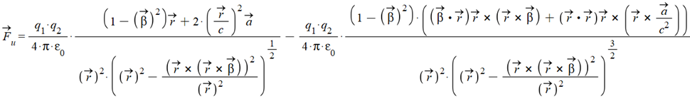
(1)
Where \vec{\beta}=\frac{\vec{v}}{c}, and \vec{r},\ \vec{v},\ \vec{a}, are the relative position, velocity, and acceleration between the two charges. In general, velocity and acceleration may not have the same direction. Let’s define their angles with respect to the vector \vec{r}.
\theta: angle between \vec{r} and \vec{v}
\alpha: angle between \vec{r} and \vec{a}
Thus, we can write the universal force in geometrical form:
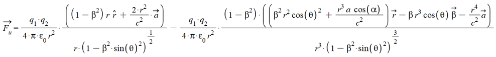
(2)
If we assume that velocity and acceleration point in the same direction of \hat{r} (\theta=\alpha=0), the magnitude of the universal force reduces to:
F_u=\frac{kq_1q_2\left(\left(1-\beta^2\right)\ r+\frac{2r^2a}{c^2}\right)}{r^3}-\frac{kq_1q_2\left(1-\beta^2\right)\left(\left(\beta^2r^2+\frac{r^3a}{c^2}\right)r-\frac{\beta r^3v}{c}-\frac{r^4a}{c^2}\right)}{r^5} (3)
Applying the second Newton law for positive charges and solving for the system mass, we obtain:
m=\frac{kq_1q_2\left(\left(1-\beta^2\right) r+\frac{2r^2a}{c^2}\right)}{a r^3}-\frac{kq_1q_2\left(1-\beta^2\right)\left(\left(\beta^2r^2+\frac{r^3a}{c^2}\right) r-\frac{\beta r^3v}{c}-\frac{r^4a}{c^2}\right)}{a r^5} (4)
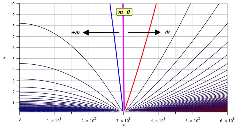
Graph of mass showing that negative mass is required for faster-than-light travel
Note that for charges of opposite sign, the acceleration will be negative, though Eq. (4) will give the same result.
In Fig. 1 we see a contour or level graph of the system mass with respect to velocity and acceleration. In this example, velocity was extended to double the speed of light (v=2c \left[\frac{m}{s}\right]), while acceleration was given an arbitrarily low maximum value of a=10 \left[\frac{m}{s^2}\right]. The purple vertical line at v=c corresponds to m=0. As expected, it is independent of the acceleration. The blue line to the left indicates the region of positive mass, while the red line on the right indicates the region of negative mass.
In order to make possible faster-than-light travel, we clearly see that mass must decrease as velocity increases and must be negative for velocities higher than the speed of light.
Unlike the flawed theory of relativity, faster-than-light travel does not violate any laws of physics.
Newton’s laws are still valid for v>c, but inverted. Acceleration points in the opposite direction of the acting force, while the reaction force points in the same direction as the acting force. In further paragraphs, we’ll see that friction and drag vanish, as they point in the same direction as the acting force too. Before examining the bases of superluminal dynamics, let’s briefly mention important flaws that make both the theory of relativity and quantum theory useless.
Main Flaws in the Invalid Theory of Relativity
More than a century of advancement in real-world physics was hindered and damaged by scientists’ blind adherence to Einstein’s unphysical theory of relativity. It is inexplicable that scientists are still squandering time nowadays creating papers based on such a theory, which violates basic laws of physics.
The fundamental fault of this theory lies precisely in the tenet of relative motion.
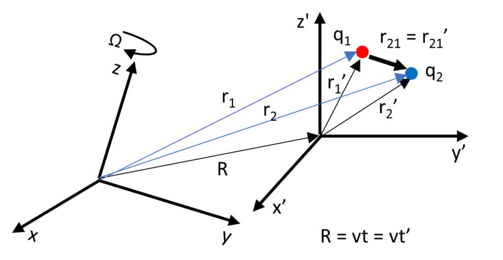
Relative motion only depends on relative coordinates
1. Relative motion depends on relative coordinates, not on reference frames.
As shown in Fig. 2, this motion is entirely relational [2], and magnitudes such as {\vec{r}}_{12},\ {\hat{r}}_{12},\ r_{12},\ {\dot{r}}_{12},\ {\ddot{r}}_{12}, will have the same value on any frame of reference.
The only magnitudes that depend on reference frames are non-relational and based on the individual magnitudes of each particle, such as:
{\vec{r}}_{1},{\vec{r}}_{2},{\vec{v}}_{1},{\vec{v}}_{2},{\vec{a}}_{1},{\vec{a}}_{2}, {\vec{v}}_{12}{=}{\vec{v}}_{1}-{\vec{v}}_{2},{\vec{a}}_{12}{=} {\vec{a}}_{1}-{\vec{a}}_{2}, {| {\vec{v}}_{12}|}{=}\sqrt{{\vec{v}}_{12}^{2}},{| {\vec{a}}_{12}|}{=} \sqrt{{\vec{a}}_{12}^{2}},{\hat{r}}_{12} {\vec{a}}_{12},{\vec{r}}_{12} {\vec{a}}_{12}This fundamental tenet of physics is sufficient to disprove the theory of relativity.
2. The speed of light is not absolute.
Einstein declared in his second postulate of special relativity: “Any ray of light moves in the “stationary” system of co-ordinates with the determined velocity c, whether the ray be emitted by a stationary or by a moving body.”
This postulate is completely ridiculous. The fundamental principles of physics that govern relative motion are also violated by this flawed and non-physical premise. Furthermore, a frame in motion and a frame at rest have different wave equations.
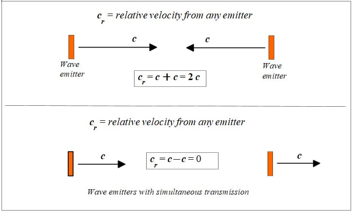
Relative motion of wave fronts between two wave sources at rest
The velocity of light is not absolute but depends on the relative motion between sources or between the source and detector (observer). See Figs. 3, 4, and 5.
That is, the speed of light obeys the principle of relative velocity addition/subtraction, which means that there is no speed limit in the universe as stated in the ill-fated theory of relativity. The velocity of an EMW source adds/subtracts to the wavefront speed. Otherwise, no Doppler effect [3] or Cherenkov effect will be observed [9].
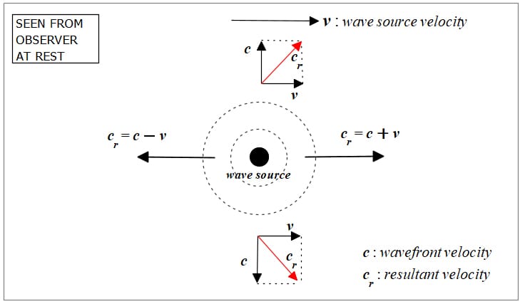
Relative motion between wavefront and a wave source as seen from an observer at rest
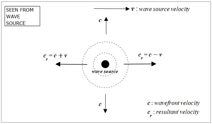
Relative motion between a wavefront and a wave source as seen from the wave source
Light velocity is not constant for all observers and is not constant with respect to the relative motion between source and observer. The velocity of a wave is constant only relative to the medium.
3. Time dilation and length contraction do not exist as physical effects.
See the classical example of a wave source sending an EMW to a mirror on the y-axis, with the system at rest in Fig. 6, and the system moving to the right with velocity v in Fig. 7, as viewed by an observer at rest. The wave reflection in mirror M is only illustrative, but not necessary for calculations.
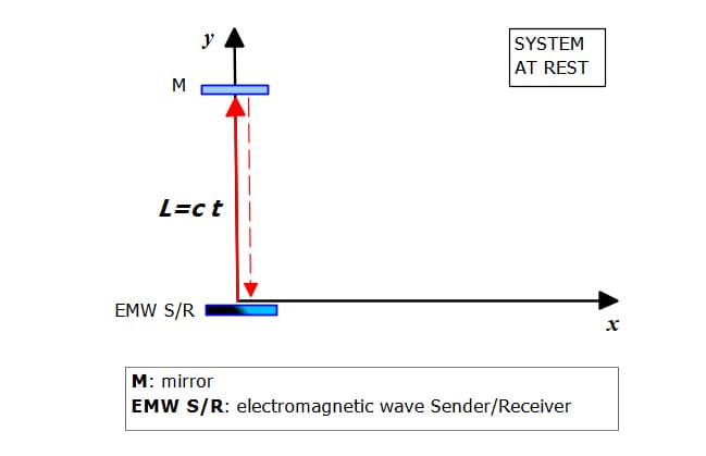
System of wave transmitter-receiver and mirror at rest
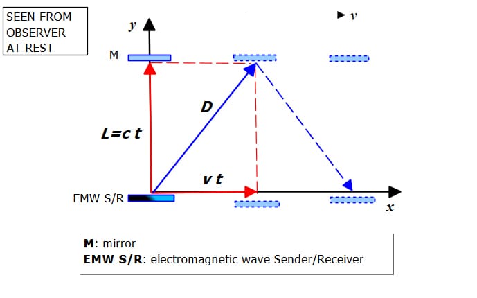
System of wave transmitter-receiver and mirror moving at velocity v as seen from an observer at rest
The time required by the wavefront to cover the distance from the sender to the mirror is t=\frac{L}{c}. This time does not change when the system is moving with velocity v to the right. The path length of light (D) as seen from an observer at rest is \mathrm{D}=\sqrt{c^2t^2+v^2t^2}=\sqrt{1+\frac{v^2}{c^2}} ct. By replacing the time, the path length seen by an observer at rest becomes \mathrm{D}=\sqrt{1+\frac{v^2}{c^2}} L; that is, the observer sees a longer path relative to the rest condition.
As Einstein postulated the absolute value of the speed of light as a limit, he had to invent a different time (or clock) to explain his flawed theory. But real-world physics dictates that if a longer distance is covered in the same time interval, the velocity must be higher than that in the short distance. There is absolutely no physical reason to assign a different time (clock) for the system at rest and in motion.
Proof that time is the same in both frames
Let’s assign time t for the system at rest L\ =c\ t and t_1=\frac{\mathrm{D}\ }{\sqrt{1+\frac{v^2}{c^2}} c} to the path length on the moving system. After replacing D in the last equation, we get t_1=t.
Proof that the speed of light is not the same in both frames
This proof is already in the equation of the path length for the system in motion \mathrm{D}=\sqrt{1+\frac{v^2}{c^2}} ct that we can write as \mathrm{D}=c_1t, where c_1=\sqrt{1+\frac{v^2}{c^2}}\ c. It is evident that c_1>c.
A longer path is naturally measured for the same time interval by the observer at rest due to the relative velocities in the motion. A longer path for the same amount of time requires a higher velocity since the laws of physics are the same everywhere. This has been demonstrated to be true.
4. Wrong Energy and Momentum formulas.
The equations of energy and momentum in the theory of relativity totally ignore one very important kinetic variable, like acceleration. As a solace of the theory of relativity, the same thing occurs in mechanical physics.
In the study “Nuclear Fusion Enhanced by Negative Mass – A Proposed Method and Device” [4], a total energy equation was derived from the Universal Electrodynamic Force. This equation is the first found in physics that really accounts for the total energy of a system and has three terms. A potential energy term, a kinetic term depending on velocity, and a kinetic term depending on acceleration, which is the radiation energy E_{rad} in a system of charges:
E=\gamma_{E}\left(U+K+E_{rad}\right), where \gamma_{E}=\frac{1}{\sqrt{1+\left(\cos^2{\left(\theta\right)}-1\right)\frac{v^2}{c^2}}}. In mechanical systems, E_{rad} can be named E_a, i.e., the energy due to the acceleration.
When Einstein’s energy equation is applied to nuclear fusion, it yields insufficient energy results and is very risky since it ignores radiation energy, which can occasionally be higher than kinetic energy. Working with nuclear fusion devices requires scientists to use extreme caution and safeguard their health.
Our equation, instead, was successfully applied in the calculation of the real released energy in the nuclear fusion reaction and the real energy of the products [4].
Also, for the first time in physics, a total momentum change formula was derived based on the Universal Electrodynamic Force. Similarly to the total energy, the momentum change equation also has a term depending on acceleration:
P=\gamma_P\left(\frac{E_0}{v}\left(1-\frac{v^2}{c^2}\right)+\frac{E_{rad}}{v}\right), where \gamma_P=\frac{1}{\sqrt{1-\sin^2{\left(\theta\right)}\cdot\frac{v^2}{c^2}}}. Again, in mechanical systems, E_{rad} can be named E_a, i.e., the energy due to acceleration. This equation was also successfully applied to nuclear fusion reactions [4].
The “relativistic” momentum equation is wrong because it entirely ignores the total energy of the system.
5. “Ripples in space-time” do not exist as physical effects.
Gravity is an EMW of atomic origin caused by dipole oscillation in the atom [5] [6]. Gravitational waves are electromagnetic waves, and space is not something mechanical that can be moved. You cannot grant geometrical properties to a force of electromagnetic origin.
Space is a concept that determines the distance among physical entities. This distance was called “void,” “ether,” etc. The space (distance) between physical entities is filled mainly by a fabric of gravitational and non-gravitational EMWs (and even cosmic particles) that keep our universe fully connected. We cannot warp space as Einstein proposed, but we can bend electromagnetic fields.
When a cosmic object explodes or collapses, a gravitational electromagnetic shock wave pulse of huge amplitude is generated. Cosmic explosions carry out colossal amounts of electromagnetic energy in the form of momentum.
This gigantic momentum pulse will shake all cosmic objects. Then, it is absolutely natural to expect a mechanical vibration and a push on them because of the huge radiation pressure.
We have an extremely sensitive interferometer on Earth that can detect the tail pulse of gravitational EMWs from cosmic cataclysms. It detects the Earth vibration caused by the momentum of the pulse (radiation pressure), not the “ripples in space-time.” Still, highly sensitive seismic instruments might also be used to detect massive cosmic explosions.
Though the first flaw mentioned above already invalidates and makes Einstein’s theory of relativity useless as a whole, other main flaws were stated to open the eyes of those who are unthinkingly following a very wrong path of a pseudo-science that cannot be called Physics.
Main Flaws in the Invalid Quantum Theory
This is another unphysical and faulty theory that contributed to hindering and damaging the right development of real-world physics for over 100 years [7] [8]. As with the theory of relativity, it is not understandable that scientists are still wasting time to date creating articles based on this theory, which violates several laws of physics and invents explanations contradicting experimental proofs.
The fundamental fault of this theory lies precisely in its foundation: the unphysical Schrödinger wave equation.
1. Unphysical, complex-valued wave function.
The real world is determined by real-valued measurements, while this theory is based on a complex-valued wave function that describes an unreal, non-physical world.
2. Wrong assumption of unphysical “point particles.”
A point has no dimensions. It does not exist. You cannot grant physical properties to it.
3. The claim of randomness and the rejection of causality.
4. Wrong atomic models that violate basic laws of electrodynamics.
5. Unphysical forces that are caused by non-material “particles” (bosons, gravitons, etc.), instead of electromagnetic fields.
6. Physical laws change according to observers.
7. No real physical explanation for the absorption and emission of electromagnetic energy by particles.
8. The laws of mechanics and electrodynamics do not hold on all size scales.
9. Unable to explain the electromagnetic origin of gravity.
These are just a few flaws among others.
The first flaw mentioned above already invalidates and makes quantum theory useless as a whole. Other significant shortcomings were mentioned, nevertheless, in order to alert those who are blindly adhering to a pseudo-science that isn’t genuine Physics.
Faster-Than-Light Travel Possible By Gravitational and Inertial Control of Mass
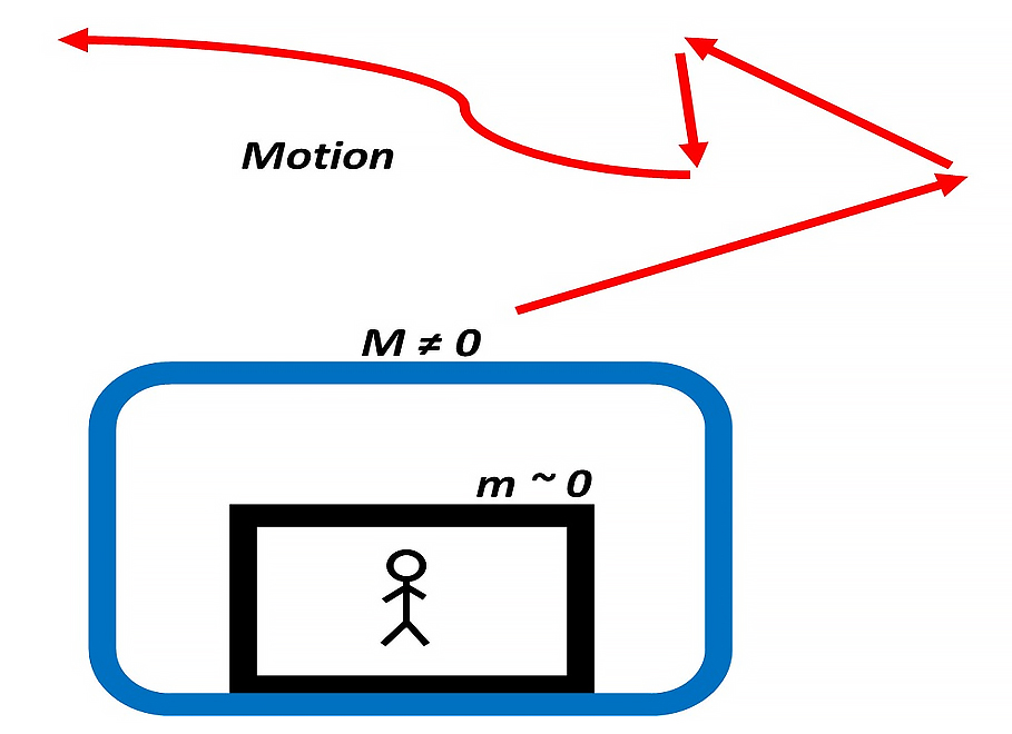
Spaceship with gravitational and inertial control working together
In the study about Negative Mass in Atom Nuclei (Part 6), it was undoubtedly demonstrated that inertial control as well gravitational control of mass are possible by applying any of the three proposed methods to obtain negative mass as mentioned in the introduction of the present work.
Imagine a spaceship with controlled mass M, of any sign and magnitude different from zero (Fig. 8). A passenger is transported in a cabin of mass m having a magnitude near zero and isolated from M.
By controlling the magnitude and sign of mass M, it is possible to achieve huge accelerations/decelerations almost instantly and change motion directions, which will defy classic physics because of the inertial effects.
However, if we keep the mass m of the passenger cabin near zero, he or she will not feel any inertial discomfort, despite the type of motion.
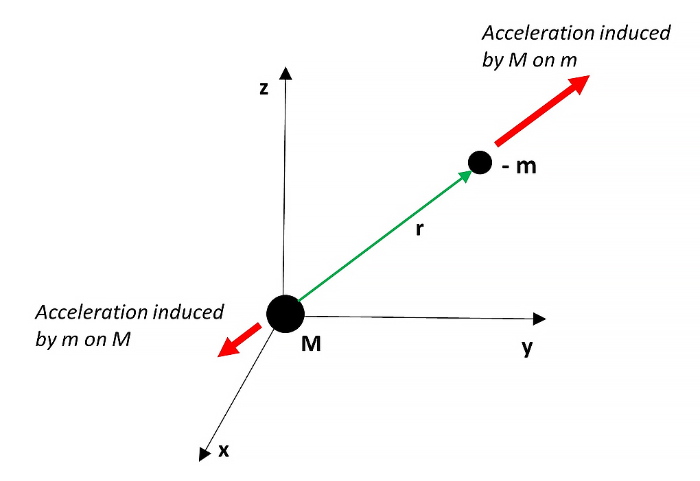
Gravitational forces between positive and negative mass
Negative mass causes a repulsive gravitational force, as shown in Fig. 9. It means that by controlling the mass magnitude and sign, we can master the gravitational field as a free energy source for propulsion.
If M>>m, the acceleration on m will have a considerable magnitude, while mass M will not perceive any effects.
By making the magnitude of the mass as small as possible, inertial effects will disappear. The linear momentum will vanish. So will the centrifugal force and the angular momentum in rotational systems.
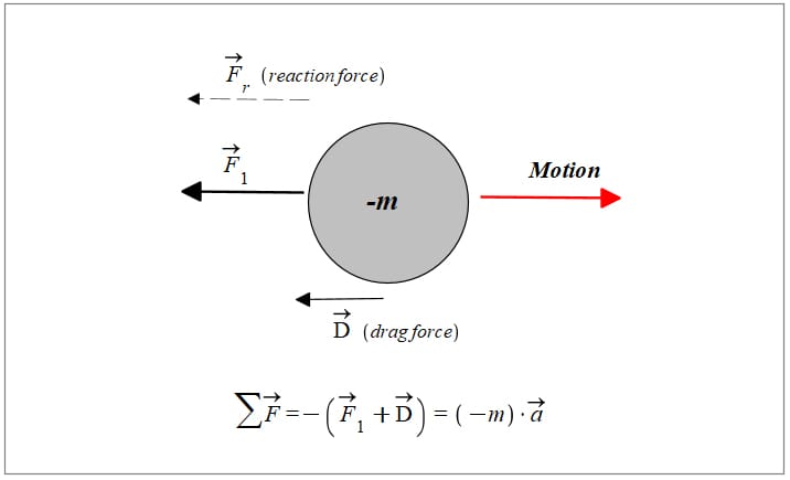
In the negative mass regime, the drag force acts in the direction of the acting force
If the spaceship in Fig. 8 has negative mass and is moving in a fluid (e.g., air or water), the drag force, instead of opposing the motion, will contribute to the propulsion force, as shown in Fig. 10.
Recall that in a negative mass regime, the direction of motion is opposite to the applied force, and that the reaction force points in the same direction as the acting force. The reaction force also contributes to the propulsion.
In the following paragraphs, the faster-than-light travel of a hypothetical spaceship as shown in Fig. 8 will be analyzed.
Faster-Than-Light Travel Example of a Spaceship to a Star in Andromeda
The study on “Negative Mass – Gravitational and Inertial Control” [1] is based on the nuclear structure of the Aluminum atom because it is an easy-to-find material for experimental purposes. It means that the structure of the hypothetical spaceship of Fig. 8 is Aluminum. We imagine that this spaceship will travel from the Earth to a distant star like the Sun located in the Andromeda galaxy.
Gravitational attraction on the spaceship caused by the COMU
The spacecraft that is going to make faster-than-light travel will have mass control by methods 2. and 3. as mentioned in the introduction of this study.
Forces on the Spacecraft Used For Faster-Than-Light Travel
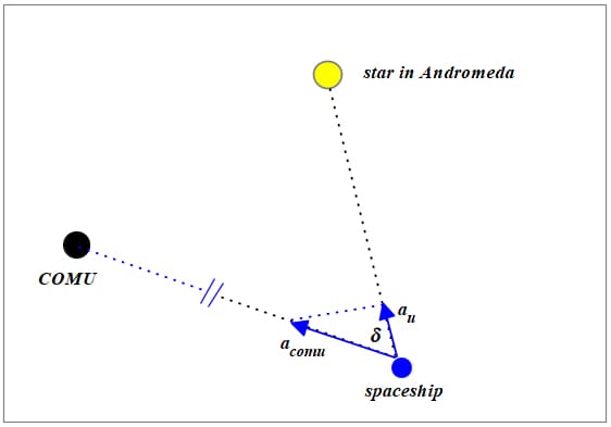
The assumed external forces acting on the spaceship will be the gravitational attraction from Earth and from the distant star, as well as an estimated fraction of the universe’s gravitational attraction a_u caused by the COMU, as shown in Fig. 11.
Assume that the mass of the universe is m_u=1.5\ {10}^{53}\ [Kg], and the distance of the spaceship to the COMU is r_{comu}={10}^{23}\ [m].
Suppose that the direction of travel makes an angle \delta=\frac{\pi}{3} with the COMU. Then, the gravitational acceleration of the universe’s mass on the spacecraft is a_u=\left(-\frac{Gm_u}{r_{comu}^2}\right)\cos{\delta}=-5\ {10}^{-4}\ [\frac{m}{s^2}].
Assume that the regular mass magnitude of the spaceship is m_s={10}^3\ [Kg]. The distance to the star in Andromeda is r_a=2\ {10}^6\ [ly]=1.89\ {10}^{22}\ [m], while the mass of the star is m_a=2\ {10}^{30}\ [Kg].
The Universal Electrodynamic Force Role in Faster-Than-Light Travel
The Universal Electrodynamic Force for radial motion is:
{\vec{F}}_u=\frac{kq_1q_2}{r^2}\left(\frac{\left(1-\beta^2\right)\ r+\frac{2r^2a}{c^2}}{r}-\frac{\left(1-\beta^2\right)\left(\left(\beta^2r^2+\frac{r^3a}{c^2}\right)r-\beta^2r^3-\frac{r^4a}{c^2}\right)}{r^3}\right)\ \hat{r} (5)
This Universal Electrodynamic Force describes the relative motion between two charges. On what follows, the charges will be replaced by the respective masses of the two bodies, i.e., the spaceship mass m_s and the star mass m_a, their sum being m_{sys}, while v and a give the relative velocity and acceleration between them.
The Sum of Forces
Applying the second Newton law, the sum of forces must be equal to the system mass m_{sys}=(m_s+m_a) times the relative acceleration between the spaceship a_s and the star a_a, a=\left(a_s-a_a\right), that is:
\Sigma F=F_u+F_{ext}=m_{sys}\ aThe external gravitational forces acting on the spacecraft are:
Where m_e is the Earth mass, m_s is the spacecraft mass, and r is the distance from the Earth surface to the star surface, which we can approximate to r=1.89\ {10}^{22}\ [m].
F_{us}=\left(-\frac{Gm_um_s}{r_{comu}^2}\right)\cos{\delta}\ \ \ \ the\ gravitational\ force\ of\ universe\ mass\ m_u\ from\ the\ COMUWe assume that both r_{comu} and the angle \delta remain constant during the journey.
As a result, we get:
After some algebra, we obtain:
{\vec{F}}_u=(m_s\left(2a_a+a_e-a_s+a_u\right)-m_a\left(a_s-a_a\right))\hat{r} (6)
Where a_e is the gravitational acceleration of Earth, a_a is the gravitational acceleration from the distant star in Andromeda, a_u is the gravitational acceleration of the universe’s mass from the COMU, m_s is the mass of the spaceship, and m_a is the mass of the distant star in Andromeda.
By equating Equations (5) and (6), we have:
\frac{kq_1q_2}{r^2}\left(\frac{\left(1-\beta^2\right)\ r\hat{r}+\frac{2r^2a\hat{r}}{c^2}}{r}-\frac{\left(1-\beta^2\right)\left(\left(\beta^2r^2+\frac{r^3a}{c^2}\right)r\hat{r}-\beta^2r^3\hat{r}-\frac{r^4a\hat{r}}{c^2}\right)}{r^3}\right)=(m_s\left(2a_a+a_e-a_s+a_u\right)-m_a\left(a_s-a_a\right))\hat{r} (7)
On the left-hand side, we have the charges instead of the masses of the spaceship and star. We need to express the charges in terms of the respective masses.
Writing Charge in Terms of Mass
The mass of a charge can be expressed as: m=\frac{q^2}{{4\pi\varepsilon}_0r_0c^2}\ [Kg], where r_0 is the radius of the charge. To calculate the radius of the charge r_0=\frac{q^2}{\varepsilon_0\ m\ c^2}\ \left[m\right], we will remove the constant 4\pi. By keeping consistency, even if the calculated radii are bigger, this won’t have an impact on the mass calculations that follow.
The new atomic model [1] predicts a high elasticity of the charges. It means that they will have different radii when they are packed in the nucleus as when they are outside the nucleus. Protons in the distant star will have a greater radius than in the Aluminum nucleus.
For simplicity, suppose that the only element making the star is Hydrogen. The total number of charges in the distant star is Q_1=N_1Z_1q_1, where N_1 is the number of atoms in the star, Z_1 is the atomic number of Hydrogen, and q_1 is the proton charge. Now let’s multiply and divide Q_1 by q_1\varepsilon_0r_{0a}c^2, where r_{0a} is the proton radius in the star:
N_1Z_1q_1\frac{q_1\varepsilon_0r_{0a}c^2}{q_1\varepsilon_0r_{0a}c^2}=\ \frac{N_1Z_1q_1^2}{\varepsilon_0r_{0a}c^2}\ \frac{\varepsilon_0r_{0a}c^2}{q_1}=m_a\frac{\varepsilon_0r_{0a}c^2}{q_1} (8)
On the other hand, the total number of charges in the Aluminum spaceship structure is Q_2=N_2Z_2q_2, where N_2 is the number of atoms in the Aluminum mass, Z_2 is the atomic number of Aluminum, and q_2 is the proton charge. Now let’s multiply and divide Q_2 by q_2\varepsilon_0r_{0s}c^2, where r_{0s} is the proton radius in the Aluminum nucleus:
N_2Z_2q_2\frac{q_2\varepsilon_0r_{0s}c^2}{q_2\varepsilon_0r_{0s}c^2}=\ \frac{N_2Z_2q_2^2}{\varepsilon_0r_{0s}c^2}\ \frac{\varepsilon_0r_{0s}c^2}{q_2}=m_s\frac{\varepsilon_0r_{0s}c^2}{q_2} (9)
Now we can replace (8) and (9) in (7) to get a homogeneous equation in terms of masses:
m_am_s\left(\frac{\varepsilon_0c^2}{q^2}\right)^2r_{0a}r_{0s}\frac{k}{r^2}\left(\frac{\left(1-\beta^2\right)\ r\hat{r}+\frac{2r^2a\hat{r}}{c^2}}{r}-\frac{\left(1-\beta^2\right)\left(\left(\beta^2r^2+\frac{r^3a}{c^2}\right)r\hat{r}-\beta^2r^3\hat{r}-\frac{r^4a\hat{r}}{c^2}\right)}{r^3}\right)=(m_s\left(2a_a+a_e-a_s+a_u\right)-m_a\left(a_s-a_a\right))\hat{r} (10)
Where q is the proton charge, r_{0a}=1.9\ {10}^{-17}\ [m] is the proton radius in the star, and r_{0s}=8.6\ {10}^{-18}\ [m] is the proton radius in the Aluminum nucleus.
Verifying the Mass of the Star
The number of Hydrogen atoms in the star and other magnitudes are:
N_1=\frac{mass\ of\ Star\ \left[g\right]}{molar\ mass\ of\ H\ \left[\frac{g}{mol}\right]}\cdot Avogadro\ number=\ 1.19\ {10}^{57}; Z_1=1; r_{0a}=1.9\ {10}^{-17}\ [m]
Verifying the Mass of the Spaceship Used For Faster-Than-Light Travel
The number of Aluminum atoms in the mass of the spacecraft and other magnitudes are:
N_2=\frac{mass\ of\ Spaceship\ \left[g\right]}{molar\ mass\ of\ Al\ \left[\frac{g}{mol}\right]}\cdot Avogadro\ number=\ 2.23\ {10}^{28}; Z_2=13; r_{0s}=8.6\ {10}^{-18}\ [m]
We see that both masses have been verified with very good approximation for the decimal places taken.
Now we can make calculations based on Eq. (10) for methods 2. and 3. as described in the introduction of this study. For a better progression, we’ll start with method 3, which offers less “drastic” results compared to method 2.
Faster-Than-Light Travel by Applying an Electric Signal Plus a Static Electric Field to the Aluminum Nucleus
We’ll apply this method to the Aluminum frame (mass M) of our hypothetical spaceship in Fig. 8. From the work on Negative Mass in Atom Nuclei – Part 5, we see that the external force applied to the Aluminum nucleus is given by Eq. (4) from that study: {\vec{F}}_{ext}=\frac{13\ q}{3}\left(E_f+E_s\cos{\left(\omega t\right)}\right)\ \hat{r}.
The results from the five calculation steps that follow are summarized in the table of Fig. 14.
Step 1 of Calculation for Faster-Than-Light Travel: nuclear mass
To make the mass independent of time, we take the Aluminum nuclear mass m_n, Eq. (8) from the reference study, and make a time average for the signal period. To facilitate the integral calculation, a Taylor series expansion of m_n to 16 terms was made before integration.
m_{avg}=\frac{1}{T}\cdot\int_{0}^{T}m_ndt=\frac{\omega}{2\pi}\cdot\int_{0}^{\frac{2\pi}{\omega}}m_ndtThen, a contour or level graph of the mass is made vs. the signal amplitude and static electric field amplitude for diverse signal frequencies, and the following nuclear parameters:
| r_n=3.5\ {10}^{-15}[m] Aluminum\ nuclear\ radius | \omega_e={10}^{15}[\frac{1}{s}]\ nuclear\ electron\ shells\ frequency |
| \omega_p={10}^{16}[\frac{1}{s}]\ nuclear\ proton\ shells\ frequency | A_e=2\ {10}^{-16}[m]\ amplitude\ of\ electron\ shell\ oscillation |
| A_p=\frac{A_e}{{10}^3}[m]\ amplitude\ of\ proton\ shell\ oscillation |
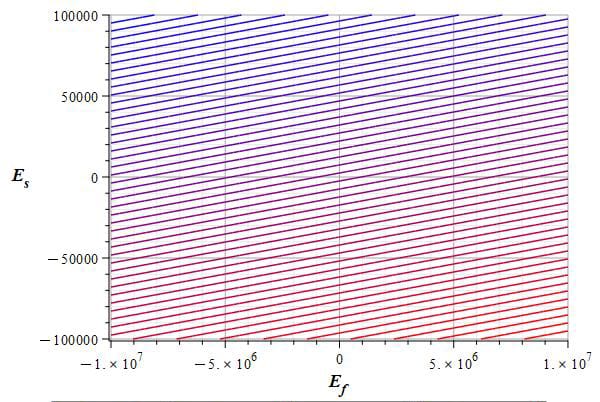
Example of a contour or level graph of the negative mass in the Aluminum nucleus due to a signal and static electric field
In Fig. 12 we see a graph example for a signal amplitude range of E_s=-{10}^5\ to\ {10}^5[\frac{V}{m}], a static electric field magnitude range of E_f=-{10}^7\ to\ {10}^7[\frac{V}{m}], and a signal frequency of \omega=1.60848\ {10}^{16}[\frac{1}{s}]. These combinations of parameters give an Aluminum nuclear mass of m_{avg}=-1.24\ {10}^{-15}[Kg].
It is obvious that this graph must be repeated each time the parameters of the signal and/or electric field change.
Step 2 of Calculation: spaceship mass, velocity and acceleration
With the result of m_{avg}, we can calculate the mass of the spaceship: m_s=N_2{\ m}_{avg} (11).
With the result given by Eq. (11), we can solve Eq. (10) for velocity v, which will be a function of a_s and r, that is, v=\pm\ f(a_s,\ r). We take the positive solution and make a level or contour graph of the relative velocity vs. the distance range between Earth and the distant star r=6.378\ {10}^6\ to\ 1.89\ {10}^{22}[m], and a spaceship acceleration range between zero and its maximum value a_s=0\ to\ max.\ value\ [\frac{m}{s^2}]. This maximum acceleration value can be calculated as follows:
The magnitude of the external force (see beginning of section) applied to the nucleus is F_{ext}=\frac{13}{3}q\ \left(E_s+E_f\right). By choosing the maximum amplitudes of the signal and static electric field, we get the maximum acceleration of the Aluminum nucleus, which will be the acceleration of the spaceship: {| a_{s}|}={| \frac{F_{\mathit{ext}}}{m_{\mathit{avg}}}|} (12).
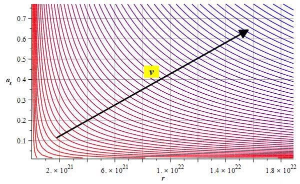
Example of a contour or level graph of the faster-than-light velocity vs. distance and acceleration by applying a signal + electric field to the Aluminum nucleus
Once we have both the distance range and the acceleration range, we can make a level or contour graph of the velocity vs. distance and acceleration, as seen in the example given in Fig. 13.
From this graph, we pick the maximum relative velocity.
As the magnitude of the relative velocities is very high, the distant star in Andromeda can be considered “at rest,” and the relative velocity is practically given only by the spaceship.
Step 3 of Calculation: time to destination
Since we assumed rectilinear, constant accelerated motion with zero initial velocity, we can now calculate the time required by the spaceship to arrive at the distant star in Andromeda: t=\pm\frac{\sqrt{{2\ a}_s\left(r-r_0\right)}}{a_s}, where r is the distance from the Earth surface to the star surface (\approx 1.89\ {10}^{22}[m]), r_0 is the Earth radius, and a_s is the maximum spacecraft acceleration.
Step 4 of Calculation: total energy
Calculation of the total energy [4] of the system, which turns out to be practically given only by the spacecraft.
E=\gamma_E\left(U+K+E_a\right). In our radial motion \gamma_E=1, and the full energy equation becomes:
E=\frac{km_am_s\varepsilon_0^2c^4r_{0a}r_{0s}}{q^2}\left(\left(\frac{1}{r_f}-\frac{1}{r_i}\right)-\frac{1}{c^2}\left(\frac{1}{r_f}-\frac{1}{r_i}\right)v^2-\frac{1}{c^2}2\left(ln{\left(r_i\right)}-ln{\left(r_f\right)}\right)a\right) (13)
Where r_i=(1.89\ {10}^{22}-6.378\ {10}^6)[m] is the distance to the star in Andromeda minus the Earth radius, and r_f=696\ {10}^6[m] is the distant star radius.
The total energy of the distant star (potential energy plus radiation energy) is approximately E_{star}=2\ {10}^{41}+(-1.75\ {10}^{38})\ \cong\ 2\ {10}^{41}[J].
The system’s energy is given by the spaceship energy plus the star energy E=E_s+E_{star}. Since in all cases we’ll have that E_s>>E_{star}, the system’s energy is practically given only by the energy of the spacecraft, that is, E\cong\ E_s.
Below follows an example of the total energy calculation and the magnitude of each term for a spaceship’s maximum velocity v=1.66\ {10}^{11}[\frac{m}{s}], acceleration a_s=0.77[\frac{m}{s^2}], and a spaceship mass of m_s=-2\ {10}^{15}[Kg]:
Step 5 of Calculation: total momentum
Calculation of the total momentum change of the system [4].
P=\frac{E_0}{v}\left(1-\frac{v^2}{c^2}\right)+\frac{E_a}{v}, where E_0 is the energy at rest, and E_a is the energy due to the acceleration; both were previously calculated above.
Below is an example of the total momentum change calculation for a spaceship’s maximum velocity v=1.66\ {10}^{11}[\frac{m}{s}], acceleration a_s=0.77[\frac{m}{s^2}], and a spaceship mass of m_s=-2\ {10}^{15}[Kg] at the distance equal to the radius of the distant star r=696\ {10}^6[m]:
Results for Faster-Than-Light Travel by Applying an Electric Signal Plus a Static Electric Field to the Aluminum Nucleus
The table below in Fig. 14 illustrates the results of the effects of negative mass on propulsion for constant signal amplitude, diverse static electric field magnitudes, and signal frequencies. We observe that this method is very sensitive regarding signal frequency, the reason why it must be very stable and precise. The spaceship data is arranged by decreasing travel time. Remember that the time required by an EMW to arrive at the star in Andromeda is 2\ {10}^{6}\ [y].
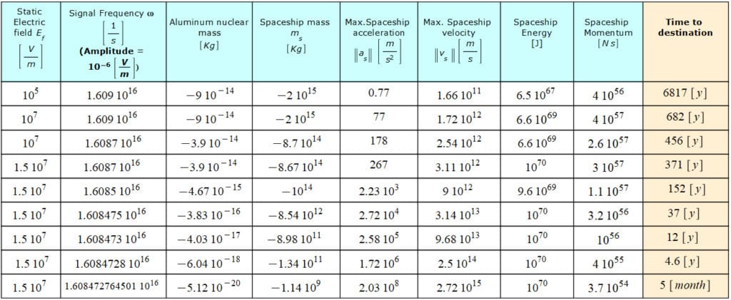
Results for Faster-Than-Light Travel by Applying an Electric Signal Plus a Static Electric Field to the Aluminum Nucleus of the spaceship structure
We can see that the fastest journeys are achieved by a static electric field magnitude of E_f=1.5\ {10}^7[\frac{V}{m}], which is almost the electrical breakdown strength of Aluminum. The range of the signal frequency lies in the extreme UV band.
Relationship Between Wave Amplitude and Wave Energy – Derived Design Parameters for the Faster-Than-Light Travel Spaceship
In the next section, we’ll analyze the other proposed method to obtain negative mass by radiating the aluminum nucleus in the spaceship’s structure by a static electric field plus an EMW. But how do we apply these fields to the structure?
The volume of the structure hit by the incident wave and the wave’s frequency will determine how much energy is needed to achieve a specific negative mass magnitude. Stated differently, it is dependent on the thickness of the structure and the incident area of the wave.
We know that the energy of a wave is proportional to its amplitude. In the study “Intensity of Electromagnetic Waves as a Function of Frequency, Source Distance and Aperture Angle” [10], it was demonstrated that a wave’s energy also depends on its frequency, in total agreement with Planck’s equation.
However, there was no equation in physics that could demonstrate it. Till now.
In the reference study [10], we defined the volumetric power (power density) as the flow of energy per unit time P_v=\frac{\partial u}{\partial t}. Then, the intensity was redefined as the volumetric energy flow per unit time per unit area I=\frac{P_v}{A}=\frac{1}{A}\ \frac{\partial u}{\partial t}\ \left[\frac{\frac{W}{m^3}}{m^2}\right]. From Eq. (21b) in the reference study, we have P_v=\varepsilon_0\omega E_{max}^2\sin{\left(2kx-2\omega t\right)}\ \left[\frac{W}{m^3}\right], where E_{max} is the maximum wave amplitude. By taking the maximum when \sin{\emptyset=1} and multiplying by the volume, we get the power P_vV=P=\frac{dE}{dt}=\varepsilon_0\omega\ E_{max}^2V\ \left[W\right]. That is, \mathit{dE} =\varepsilon_{0} \omega E_{\max}^{2} V \mathit{dt}. We integrate the expression for the wave period of the right-hand term \int_{0}^{E}dE=\int_{0}^{\frac{2\pi}{\omega}}{\varepsilon_0\omega E_{max}^2Vdt}. This gives us the equation relating the energy E with the wave amplitude E_{max} and the stricken volume V:
E=2\pi\varepsilon_0E_{max}^2V (13a).
Solving Eq. (13a) for E_{max}, we get E_{max}=\sqrt{\frac{E}{2\ \pi\ \varepsilon_0\ V}}, where the volume can be replaced by the area of the incident wave times the distance traveled by the wave in a certain thickness of the medium V=A\ d, so that E_{max}=\sqrt{\frac{E}{2\ \pi\ \varepsilon_0\ A\ d}}. Since we are dealing with a metal, we must get rid of \varepsilon_0 by multiplying and dividing by \mu_0. Then we get E_{max}=c\ \sqrt{\frac{E\ \mu_0}{2\ \pi\ A\ d}}. As a last step, we replace energy with Planck’s equation E=h\ f, which gives us the final equation relating wave amplitude with energy (frequency) in the radiated volume of a medium:
E_{max}=c\ \sqrt{\frac{h\ f\ \mu_0}{2\ \pi\ A\ d\ }} (13b)
Where E_{max} is the maximum wave amplitude, c is the speed of light, h is the Planck constant, A is the incident area of the wave on the medium, d is the thickness of the medium, and \mu_0 is the permeability of vacuum.
The wave amplitude becomes weaker for larger volumes provided the incident energy (frequency) remains constant. We may use the variables in Eq. (13b) for calculating some of the spaceship’s design parameters.
It is not a good idea to apply an EMW to the entire spaceship structure with a single source because it may be challenging to produce the required energy. Dividing the spacecraft’s interior surface into small, honeycomb-shaped radiating sections could be an approach to lessen the wave’s area of incidence for the specified thickness.
This strategy may assist us in achieving the required mass variation of the spaceship’s structure by allowing us to manage the design parameters and generate the most suitable wave amplitudes and operating frequencies.
Example of the wave amplitudes used in the table of Fig. 17
The minimum example frequency is \omega_{min}=1.05\ {10}^{19}\left[\frac{1}{s}\right], which gives an energy of E=1.1\ {10}^{-15}\ \left[J\right]. The maximum example frequency is \omega_{max}=4.8\ {10}^{19}\left[\frac{1}{s}\right], which gives an energy of E=5.06\ {10}^{-15}\ \left[J\right]. Suppose that we radiate the whole spacecraft volume with one wave source, and let’s calculate the highest wave amplitude range. The volume of the spaceship is V=0.37\ \left[m^3\right]. Then, the maximum wave amplitude for the minimum frequency is E_{max}\approx7.3\ {10}^{-3}\left[\frac{V}{m}\right], while the maximum wave amplitude for the maximum frequency is E_{max}\approx16\ {10}^{-3}\left[\frac{V}{m}\right].
It is obvious that we can choose lower or higher wave operating frequencies. The combination of variables has no limit.
Faster-Than-Light Travel by Applying a Transverse Polarized Electromagnetic Wave (TEM) plus Static Electric Field to the Aluminum Nucleus
We’ll apply this method to the Aluminum frame (mass M) of our hypothetical spaceship in Fig. 8. From the work on Negative Mass in Atom Nuclei – Part 4, we see that our selected external force applied to the Aluminum nucleus is given by Eq. (4) from that study, which now is a bit more complicated than in the former case:
F_{ext}=\frac{2\pi\varepsilon_0v_w}{3c\ K^3r_n}\cdot\left(-\frac{3E_m^2\sin{\left(2Kr_n-2\omega t\right)}}{8}-12E_fE_m\sin{\left(Kr_n-\omega t\right)}+\frac{3E_m^2\left(K^2r_n^2-\frac{1}{2}\right)\sin{\left(2\omega t\right)}}{4}+\frac{3E_m^2r_nK\cos{\left(2\omega t\right)}}{4}+6E_fE_m\left(K^2r_n^2-2\right)\sin{\left(\omega t\right)}+r_n\left(12E_fE_m\cos{\left(\omega t\right)}+K^2r_n^2\left(E_f^2+\frac{E_m^2}{2}\right)\right)K\right)
The results from the five calculation steps that follow are summarized in the tables of Figs. 17, 17a, 17b, 17c, and 17d.
Step 1 of Calculation for Faster-Than-Light Travel: nuclear mass
To make the mass independent of time, we take the Aluminum nuclear mass m_n, Eq. (8) from the reference study, and make a time average for the wave period. To facilitate the integral calculation, a Taylor series expansion of m_n to 14 terms was made before integration.
m_{avg}=\frac{1}{T}\cdot\int_{0}^{T}m_ndt=\frac{\omega}{2\pi}\cdot\int_{0}^{\frac{2\pi}{\omega}}m_ndtThen, a contour or level graph of the mass is made vs. the wave amplitude and static electric field amplitude for diverse wave frequencies, and the following nuclear parameters:
| r_n=3.5\ {10}^{-15}[m]\ Aluminum\ nuclear\ radius | \omega_e={10}^{15}[\frac{1}{s}]\ nuclear\ electron\ shells\ frequency |
| \omega_p={10}^{16}[\frac{1}{s}]\ nuclear\ proton\ shells\ frequency | A_e=2\ {10}^{-16}[m]\ amplitude\ of\ electron\ shell\ oscillation |
| A_p=\frac{A_e}{{10}^3}[m]\ amplitude\ of\ proton\ shell\ oscillation | K=\frac{\omega}{v_w}[\frac{1}{m}]\ the\ wave\ vector, where v_w is the wave velocity in the nucleus and \omega is the wave frequency. |
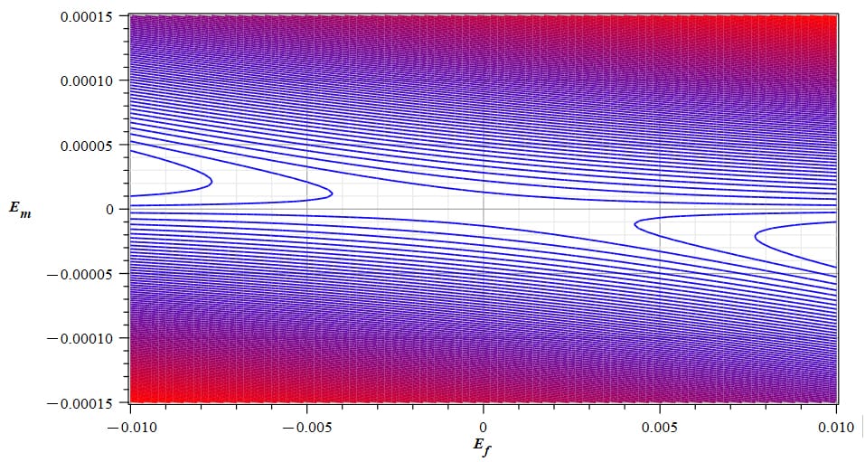
Example of a contour or level graph of the negative mass in the Aluminum nucleus due to a wave and static electric field
In Fig. 15 we see a graph example for a wave amplitude range of E_m=-1.5\ {10}^{-4}\ to\ {1.5\ 10}^{-4}[\frac{V}{m}], a static electric field magnitude range of E_f=-{10}^{-2}\ to\ {10}^{-2}[\frac{V}{m}], and a wave frequency of \omega=1.05\ {10}^{19}[\frac{1}{s}]. Let’s pick from the graph the higher negative magnitude of Aluminum nuclear mass, which in this case is m_{avg}=-284[Kg].
It is obvious that this graph must be repeated each time the parameters of the wave and/or electric field change.
Step 2 of Calculation: spaceship mass, velocity and acceleration
With the nuclear parameters and the same wave and electric field parameters as above, we calculate the external force F_{ext} (see the beginning of the section) exerted on the Aluminum nucleus by the wave and electric field.
To make the force independent of time, we take Eq. (4) from the reference study and make a time average of F_{ext} for the wave period. To facilitate the integral calculation, a Taylor series expansion of F_{ext} to 20 terms was made before integration.
F_{extAvg}=\frac{1}{T}\cdot\int_{0}^{T}F_{ext}dt=\frac{\omega}{2\pi}\cdot\int_{0}^{\frac{2\pi}{\omega}}F_{ext}dtNow we can calculate the acceleration of the spaceship: {| a_{s}|}={| \frac{F_{\mathit{extAvg}}}{m_{\mathit{avg}}}|}.
With the result of m_{avg}, we can calculate the mass of the spaceship: m_s=N_2{\ m}_{avg} (14).
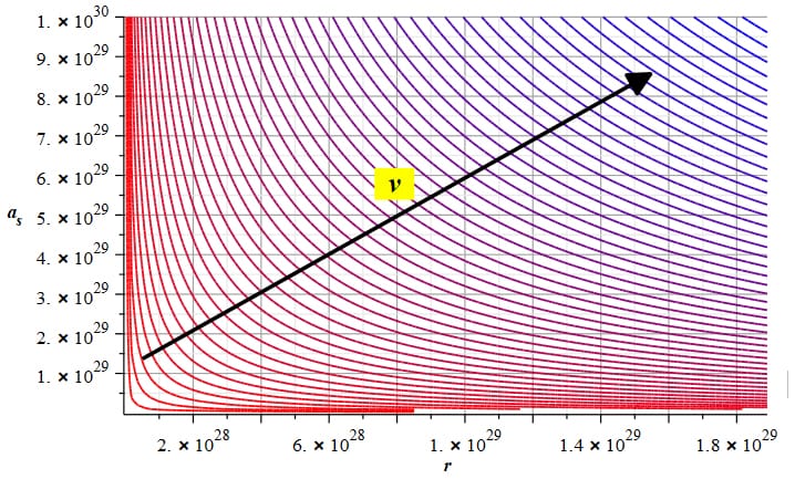
Example of a contour or level graph of the faster-than-light velocity vs. distance and acceleration by applying a wave + electric field to the Aluminum nucleus
With the result given by Eq. (14), we can solve Eq. (10) for velocity v, which will be a function of a_s and r, that is, v=\pm\ f(a_s,\ r).
We take the positive solution and make a level or contour graph of the relative velocity vs. the distance range between Earth and the distant star r=6.378\ {10}^6\ to\ 1.89\ {10}^{22}[m] and the spaceship acceleration range between zero and its maximum value a_s=0\ to\ max.\ value\ [\frac{m}{s^2}] as given above. See the graph example in Fig. 16. From this graph, we pick the maximum relative velocity.
As the magnitude of the relative velocities is very high, the distant star in Andromeda can be considered “at rest,” and the relative velocity is practically given only by the spaceship.
Step 3 of Calculation: time to destination
Since we assumed rectilinear, constant accelerated motion with zero initial velocity, we can now calculate the time required by the spaceship to arrive at the distant star in Andromeda: t=\pm\frac{\sqrt{{2\ a}_s\left(r-r_0\right)}}{a_s}, where r is the distance from the Earth surface to the star surface (\approx 1.89\ {10}^{22}[m]), r_0 is the Earth radius, and a_s is the maximum spacecraft acceleration.
Step 4 of Calculation: total energy
Calculation of the total energy [4] of the system, which turns out to be practically given only by the spacecraft.
E=\gamma_E\left(U+K+E_a\right). In our radial motion \gamma_E=1, and the full energy equation becomes:
E=\frac{km_am_s\varepsilon_0^2c^4r_{0a}r_{0s}}{q^2}\left(\left(\frac{1}{r_f}-\frac{1}{r_i}\right)-\frac{1}{c^2}\left(\frac{1}{r_f}-\frac{1}{r_i}\right)v^2-\frac{1}{c^2}2\left(ln{\left(r_i\right)}-ln{\left(r_f\right)}\right)a\right) (15)
Where r_i=(1.89\ {10}^{22}-6.378\ {10}^6)[m] is the distance to the star in Andromeda minus the Earth radius, and r_f=696\ {10}^6[m] is the distant star radius.
The total energy of the distant star (potential energy plus radiation energy) is approximately E_{star}=2\ {10}^{41}+(-1.75\ {10}^{38})\ \cong\ 2\ {10}^{41}[J].
The system’s energy is given by the spaceship energy plus the star energy E=E_s+E_{star}. Since in all cases we’ll have that E_s>>E_{star}, the system’s energy is practically given only by the energy of the spacecraft, that is, E\cong\ E_s.
Follows below an example of the total energy calculation and the magnitude of each term for a spaceship’s maximum velocity v=9\ {10}^{28}[\frac{m}{s}], acceleration a_s=2.2\ {10}^{28}[\frac{m}{s^2}], and a spaceship mass of m_s=–9.6\ {10}^{34}[Kg]:
Step 5 of Calculation: total momentum
Calculation of the total momentum change of the system [4].
P=\frac{E_0}{v}\left(1-\frac{v^2}{c^2}\right)+\frac{E_a}{v}, where E_0 is the energy at rest, and E_a is the energy due to the acceleration; both were previously calculated above.
Follows below an example of the total momentum change calculation for a spaceship’s maximum velocity v=9\ {10}^{28}[\frac{m}{s}], acceleration a_s=2.2\ {10}^{28}[\frac{m}{s^2}], and a spaceship mass of m_s=-9.6\ {10}^{34}[Kg] at the distance equal to the radius of the distant star r=696\ {10}^6[m]:
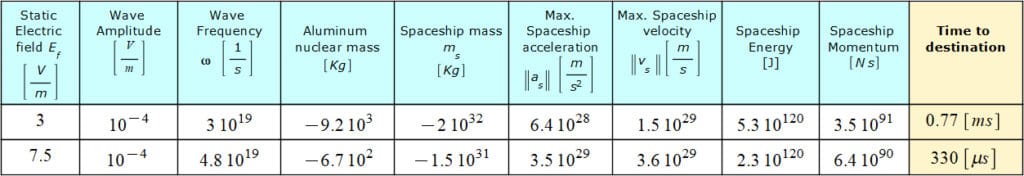
Results for Faster-Than-Light Travel by Applying a Transverse Polarized Electromagnetic Wave (TEM) plus Static Electric Field to the Aluminum Nucleus
The table below in Fig. 17 illustrates the results of the effects of negative mass on propulsion for diverse static electric field magnitudes, wave amplitudes, and wave frequencies. This method seems to be a good choice since it allows a great range of control. The spaceship data is arranged by decreasing travel time. Remember that the time required by an EMW to arrive at the star in Andromeda is 2\ {10}^{6}\ [y].
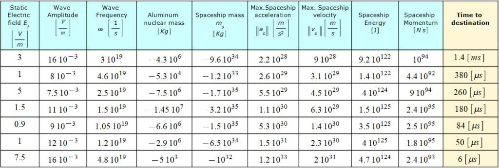
Results for Faster-Than-Light Travel by Applying an Electromagnetic Wave Plus a Static Electric Field to the Aluminum Nucleus of the spaceship structure
The range of the example wave frequency corresponds to X-ray radiation.
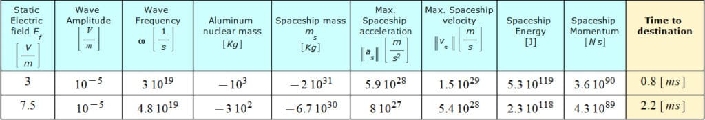
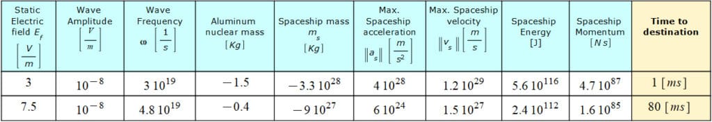
The examples shown in Figs. 17a, 17b, and 17c have the same magnitudes of static electric field and wave frequency as the first and last rows in Fig. 17. Only the amplitude of the wave was modified to observe and compare the other magnitudes.
Results for Faster-Than-Light Travel by Applying an Electromagnetic Wave of of 0.1 mV/m Amplitude Plus a Static Electric Field to the Aluminum Nucleus. To be compared with the first and last row of Fig. 17
Results for Faster-Than-Light Travel by Applying an Electromagnetic Wave of 10 µV/m Amplitude Plus a Static Electric Field to the Aluminum Nucleus. To be compared with the first and last row of Fig. 17
Results for Faster-Than-Light Travel by Applying an Electromagnetic Wave of 0.01 µV/m Amplitude Plus a Static Electric Field to the Aluminum Nucleus. To be compared with the first and last row of Fig. 17
Results by Applying a Very Low Amplitude Transverse Polarized Electromagnetic Wave (TEM) plus Static Electric Field to the Aluminum Nucleus
Some results of negative mass on propulsion are shown in the table below in Fig. 17d for a constant, much lower wave amplitude compared to those in Fig. 17. The spaceship data is arranged by decreasing travel time. Remember that the time required by an EMW to arrive at the star in Andromeda is 2\ {10}^{6}\ [y].
Results for Faster-Than-Light Travel by Applying a Very Low Amplitude Electromagnetic Wave Plus a Static Electric Field to the Aluminum Nucleus of the spaceship structure
The range of wave frequency goes from extreme-UV to X-ray radiation.
The static electric field magnitude was limited to a maximum of E_f=1.5\ {10}^7[\frac{V}{m}], which is almost the electrical breakdown strength of Aluminum.
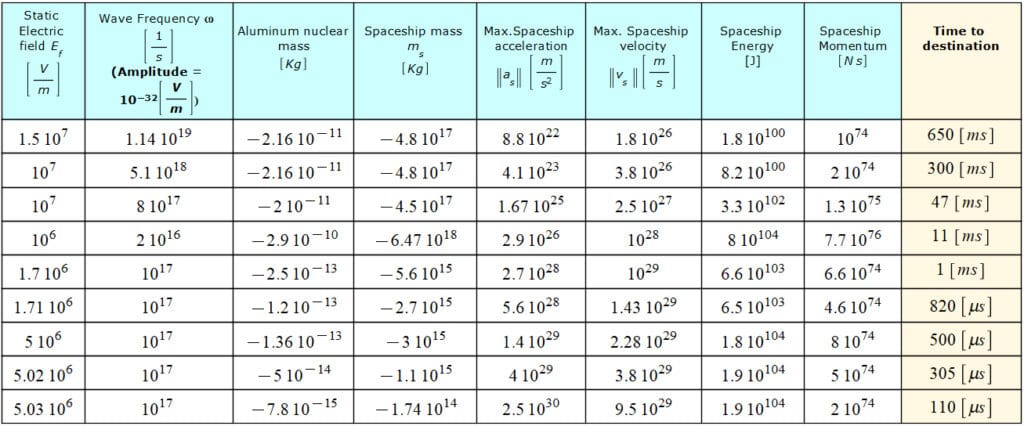
Results by Applying a High Amplitude Transverse Polarized Electromagnetic Wave (TEM) plus Static Electric Field to the Aluminum Nucleus
Other results of negative mass on propulsion are shown in the table below in Fig. 17e for much higher wave amplitudes than those in Fig. 17. The spaceship data is arranged by decreasing travel time. Remember that the time required by an EMW to arrive at the star in Andromeda is 2\ {10}^{6}\ [y].
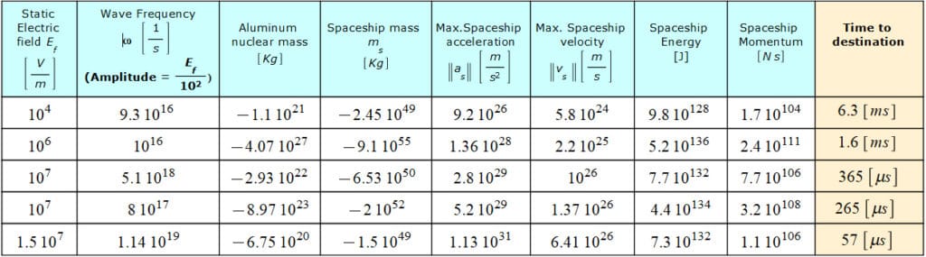
Results for Faster-Than-Light Travel by Applying a High Amplitude Electromagnetic Wave Plus a Static Electric Field to the Aluminum Nucleus of the spaceship structure
The range of wave frequency goes from UV to X-ray radiation. The static electric field magnitude was limited to a maximum of E_f=1.5\ {10}^7[\frac{V}{m}], which is almost the electrical breakdown strength of Aluminum.
The intensity attenuation of the wave in matter is approximately given by the following equation: I_{(d)}=I_{0\ }e^{-\eta\ d}, where I_0 is the intensity of the incident wave, I_{(d)} is the intensity of the wave after travelling a distance d in the matter, and \eta is the attenuation coefficient of the material, which in this case is Aluminum.
It is particularly important to bear in mind that the wave must be sufficiently powerful to penetrate into the spaceship’s aluminum frame but not so powerful as to break the aluminum nucleus. For the spaceship to operate properly, these design variables need to be carefully balanced.
Traveling a distance of \sim 2\ {10}^6[ly] in a few microseconds is a kind of teleportation, but without any need for “dematerialization.” We might be able to cross the entire universe in a few milliseconds.
How to Stop the Spaceship? – Energy, Power Release, and Momentum Change
At first look, it appears like stopping the spaceship would be difficult due to the enormous amount of energy and momentum it has developed. But the brake maneuver turns out to be rather easy because we have control over the mass.
Simply setting the mass to zero or bringing its magnitude as near to zero as feasible will bring the spaceship to a sudden stop.
Stopping Energy Example for Faster-Than-Light Travel
Let’s take the data of velocity and acceleration from the second row of the table in Fig. 17e, and suppose we abruptly change the mass of the spaceship from m_s=-9.1\ {10}^{55}[Kg] to m_s=-{10}^{-85}[Kg] when we are arriving at the destination. Check below the magnitudes of the terms in the energy and the total energy:
Power Released During the Stop Period for Faster-Than-Light Travel
Assume that we want to stop the spaceship in a time interval of t={10}^{-4}[s]. The power released by the spacecraft is P=\frac{E}{t}=575[mW].
Stopping Momentum Example for Faster-Than-Light Travel
By taking the same parameters in the energy calculation above, the total momentum change during the stop of the spaceship is:
It is evident that the spaceship comes to a sudden stop.
Effect of Gravitational Interaction Between the Spaceship and Celestial Bodies
We’ll use the table results in Fig. 17e, which were calculated for high wave amplitudes, to examine the gravitational effects that faster-than-light travel might cause. With current technology, we might not be able to generate waves with such amplitudes in that frequency range at present, but perhaps it’s possible in the future. We will make some calculations to show the gravitational effects that our hypothetical spaceship might exert on celestial bodies and how to handle them, accepting that this technology is feasible.
A repulsive gravitational force is caused by negative mass, as we already know. As we see in Fig. 17e, the spaceship might have a negative mass magnitude comparable to that of a galaxy or even nearly equal to the mass of the cosmos. Because it will create a massive, repulsive gravitational force on celestial objects located a certain distance from the ship’s path, this is extremely dangerous.
Examples of Gravitational Effects for Faster-Than-Light Travel
Let’s suppose that the wave amplitudes of Fig. 17e are technologically possible to achieve and make some calculations as examples.
As a reference, the gravitational force between the Sun and Earth is F=-3.54\ {10}^{22}[N]. Here both accelerations point towards each other and are considered positive by convention to match the relative acceleration between the objects: a=\left(a_1-\left({-a}_2\right)\right)=\left(a_1+a_2\right).
1) Let’s take the spaceship mass magnitude from the second row of the table in Fig. 17e and assume that the spacecraft fly by at a distance from Earth equal to the Earth-Moon distance. The gravitational repulsive force between Earth and the spaceship will be F=2.5\ {10}^{53}[N]. Here both accelerations point away from each other and are considered negative by convention to match the relative acceleration between the objects: a_{12}=\left(\left({-a}_1\right)-\left(a_2\right)\right)=-\left(a_1+a_2\right).
The acceleration induced by Earth on the spaceship is: a_{Es}=-\frac{Gm_E}{r^2}=-2.76\ {10}^{-3}[\frac{m}{s^2}]. As this acceleration (force) is acting on a negative mass, it will push the spaceship a bit away.
On the other hand, the large acceleration induced by the spaceship on Earth will push Earth away: a_{sE}=-\frac{Gm_s}{r^2}=4.2\ {10}^{28}[\frac{m}{s^2}]. So, we can say goodbye to the Earth!
2) Assume that the spaceship is now flying at a distance from Earth approximately from that of the Oort belt, r=5\ {10}^{14}[m]. The gravitational repulsive force between Earth and the spaceship will be F=1.45\ {10}^{41}[N]. Here both accelerations point away from each other and are considered negative by convention to match the relative acceleration between the objects: a=\left(\left({-a}_1\right)-\left(a_2\right)\right)=-\left(a_1+a_2\right).
The acceleration induced by Earth on the spaceship will not affect it: a_{Es}=-\frac{Gm_E}{r^2}=-1.6\ {10}^{-15}[\frac{m}{s^2}]. However, the huge acceleration induced by the spaceship on Earth will still push Earth away: a_{sE}=-\frac{Gm_s}{r^2}=2.4\ {10}^{16}[\frac{m}{s^2}]. Again, we can say goodbye to the Earth!
This issue is not limited to the Earth, which was chosen as a point of reference in the calculations. The entire solar system and Milky Way will be impacted by the spaceship mass.
At first sight, it seems that faster-than-light travel is not exempt from problems, and the effects of gravitational interactions are of such a magnitude that they might cause cosmic cataclysms. A carefully studied “flight plan” is imperative before starting any journey.
However, because we are traveling so quickly—far faster than the speed of light, which is the velocity at which gravity waves propagate—we really ignore the possibility that those gravitational effects could actually occur. Maybe nothing significant happens, or maybe there’s some microsecond-long gravitational shock wave. We cannot be sure. Experiments are the only way to find out.
How to Minimize Possible Gravitational Effects in Faster-Than-Light Travel
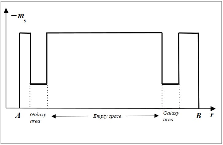
Example of mass control during faster-than-light travel between two points across two galaxies
To minimize possible gravitational effects caused by faster-than-light travel when moving inside or through a galaxy, we must reduce the mass magnitude of the spaceship to avoid dangerous interactions that may harm the free motion of celestial bodies.
A basic idea is shown in Fig. 18. If we want to travel from point A to point B, we need to go through two galaxies.
It means we must reduce the mass magnitude in those regions to avoid dangerous gravitational effects on celestial bodies belonging to those galaxies.
Once we are cleared from celestial bodies at the boundaries of the galaxies, we enter a “free space” zone where we can freely apply a “mass pulse” to gain maximum acceleration and velocity.
Collision Effects in Faster-Than-Light Travel
When you see the magnitudes of energy and momentum acquired in faster-than-light travel, no examples are needed to realize the level of destruction that a collision under this condition can cause. Here, we are talking about cosmic cataclysms caused by collisions.
The use of this technology for evil purposes will be nonsense because no lives or natural resources in entire celestial bodies or even galaxies will remain.
Regarding a regular journey, the spaceship will exert a repulsive force on obstacles due to the negative mass. However, as we are talking about a faster-than-light motion where the travel may take microseconds, we really ignore what will happen. Again, experiments will give some answers to this.
Faster-Than-Light Travel Allows Instant Cosmic Communications
The extremely short time required to connect two incredibly far-flung locations in the universe might usher in a new era for both how humankind can travel throughout the cosmos and how we can practically communicate instantly. The use of electromagnetic waves for communication will become archaic.
We might have the ability to move a type of holographic, video, or audio recorder/player back and forth between two locations in the universe. We will be able to establish live stream communications without any delay everywhere in the cosmos by moving such a device back and forth at a certain repetition frequency.
Depending on the technology we utilize at the time, we might even move a printer back and forth to print messages instantly in a variety of media.
What Else Might We Do with Negative Mass?
The primary benefit is in propulsion, as demonstrated by the current study. This will transform how we travel in cities, globally, even in the cosmos. We can instantly be anywhere we wish to be. There will be no longer need for cars, buses, trains, airplanes, ships, etc. A clean environment will be maintained. All we have to do is learn to use the gravitational field, which Mother Nature gifted us. An endless and free-to-use supply of energy.
- As stated in the preceding section, the communications sector will see the other significant improvements.
- In addition, we could lift any weight and carry it to any location with our hypothetical spaceship.
- Changes in the gravitational field will move tools or machines that need motion to perform tasks. One could set the motion endlessly.
- We might construct enclosed spaces with a specific gravity acceleration to conduct biological research or even cure particular diseases.
- Etc, etc, etc…
The inertial and gravitational control of mass opens up a limitless number of potential applications. All we have to do is exercise our imagination once this technology becomes available.
Considerations Regarding Material Subject to Mass Control
The aluminum atom’s nucleus serves as the basis for the research of negative mass in atom nuclei [1] since it is a readily available material that can be utilized experimentally to verify the theory. It takes a significant amount of energy to generate interaction effects due to the nuclear shells’ dense packing arrangement. Both the wave’s or signal’s frequency and the strength of the external fields must provide the necessary energy for faster-than-light travel. This required energy is a material’s nuclear property.
Less energy will be needed if we can use lighter metals like Lithium or Magnesium that have a simpler nuclear structure than Aluminum. However, before deciding upon using them, their mechanical properties and chemical stability need to be carefully analyzed.
It will be better to control mass by employing a single material rather than alloys. The mass control material in an alloy will be subject to strong forces that the other materials won’t be, resulting in differential forces that could potentially destroy the structure.
We might be able to develop alloys or perhaps metamaterials with the required properties to get beyond the constraints of the negative mass operating conditions in these types of compositions. Additional research and testing in laboratories will be necessary.
Experiments are needed to validate any theory. And to make things happen.
Conclusions
It has been demonstrated that the necessary condition for faster-than-light travel is negative mass.
It was proven that mass must decrease as velocity increases and must be negative beyond the speed of light.
Proof was given that there is no speed limit in the universe, as the faulty theory of relativity states.
With simple physical laws, it was proven that the speed of light is not absolute.
We stated once more that relative motion depends on relative coordinates, not on reference frames.
A few basic laws were examined that make Einstein’s theory of relativity and quantum theory totally invalid and useless.
Blindly following unphysical Einstein’s theory of relativity and quantum theory by scientists hindered and harmed more than 100 years of evolution in the development of real-world physics.
Gravitational and inertial control of mass has been demonstrated to be the basis of faster-than-light travel.
To demonstrate that traveling faster than light might be possible, a hypothetical spaceship was described, and realistic physical calculations were made.
Two methods to control the mass magnitude and sign of the spaceship were detailed, having advantages and disadvantages to each other.
It was demonstrated that faster-than-light travel can be done at extremely high velocities, which allows us to cross the entire universe in milliseconds.
Energy, power, and momentum change were calculated as examples and carefully analyzed for safety.
The possible effect of gravitational interaction between the spaceship and celestial bodies, as well as collision effects, has been analyzed.
The application of faster-than-light travel technology to instantaneous cosmic communication has been proposed.
Other possible applications of negative mass were also proposed by using the free energy of the gravitational field.
Bibliography
[1]. Raul Fattore, “Negative Mass and Negative Refractive Index in Atom Nuclei – Nuclear Wave Equation – Gravitational and Inertial Control” (2023), Part 1, Part 2, Part 3, Part 4, Part 5, Part 6
[2]. A. K. T. Assis, “Relational Mechanics and Implementation of Mach’s Principle with Weber’s Gravitational Force” (Apeiron, Montreal, 2014). http://www.ifi.unicamp.br/~assis/Relational-Mechanics-Mach-Weber.pdf
[3]. Klinaku, Shukri & Syla, et al, (2020), “Measurement of the relative velocity between an electromagnetic wave and its source/observer using the Doppler effect”. https://www.researchgate.net/publication/344840040-Measurement-of-the-relative-velocity-between-an-electromagnetic-wave-and-its-sourceobserver-using-the-Doppler-effect
[4]. Raul Fattore, “Nuclear Fusion Enhanced by Negative Mass – A Proposed Method and Device” (2024), Part 1, Part 2, Part 3, Part 4
[5]. Charles W. Lucas, Jr., “The Electrodynamic Origin of the Force of Gravity” (2008-2009), Part-1, Part-2, Part-3
[6]. A. K. T. Assis, “Gravitation as a Fourth Order Electromagnetic Effect”, Advanced Electromagnetism: Foundations, Theory and Applications, T. W. Barrett and D. M. Grimes (eds.), (World Scientific, Singapore, 1995). https://www.ifi.unicamp.br/~assis/gravitation-4th-order-p314-331(1995).pdf
[7]. Charles W. Lucas, Jr., “A New Foundation for Modern Physics” (2001), https://physics-answers.com/wp-content/uploads/2025/03/New-Foundation-for-Modern-Physics-Electron-Quantum-Mechanics.pdf
[8]. David L. Bergman, “Commentary on Sub-Quantum Physics” (2010), https://physics-answers.com/wp-content/uploads/2025/03/Commentary-on-Sub-Quantum-Physics.pdf
[9]. Raul Fattore, “Charge Radiation Derived from the Universal Electrodynamic Force – Proof of the Cherenkov Effect” (2024), https://physics-answers.com/charge-radiation-derived-from-the-universal-electrodynamic-force-proof-of-the-cherenkov-effect/
[10]. Raul Fattore, “Intensity Of Electromagnetic Waves As a Function Of Frequency, Source Distance and Aperture Angle” (2022), https://physics-answers.com/intensity-of-electromagnetic-waves-as-a-function-of-frequency-source-distance-and-aperture-angle/
Related articles:
Nuclear Fusion Enhanced by Negative Mass – A Proposed Method and Device
Charge Radiation Derived from the Universal Electrodynamic Force – Proof of the Cherenkov Effect
Intensity Of Electromagnetic Waves As a Function Of Frequency, Source Distance and Aperture Angle